Last time I argued the field is moving from one monolithic brain to a system of parts, and ended on a question I couldn’t answer: internalize the kernel, externalize the rest, but a kernel of what, and how does anything move inside the weights at all? This post is about a line of work that takes the “how” literally. It does not internalize a fact or a skill. It internalizes the loop.
My previous post ended on an unfinished thought. It argued that the 2026 frontier had quietly stopped scaling one all-purpose model and started composing a system: functional partitions instead of a single brain, acquired methodology (harness, skills, memory, tools) instead of innate scale. Underneath both axes ran a quieter question I called the most interesting one in the field. When a capability lives outside the weights, in a harness, a tool, a note, does it ever move inside, and should it? I gave a partial answer: internalize the load-bearing kernel, keep a notebook for the rest. And I named the kernel, loosely, as a world model plus the control loop that runs over it. Then I ran out of road: I had no mechanism for how a control loop becomes weights.
This post is about the mechanism. A small, fast-moving line of work has one premise: internalize not a fact and not a skill, but the loop itself: the iterative “think again, search again, revise the guess” process that we currently buy with chain-of-thought tokens or bolt on with an external scaffold. The papers are unglamorous and tiny. One of them is 7 million parameters. And they keep doing something that should not be possible, like beating o3-mini-high on ARC-AGI-1 with 27 million parameters and a thousand training examples and no pretraining at all. They are the clearest existence proof I have seen that the adaptive loop can live in the weights.
I came at them with a bet I had already made in public, before I read most of this work. The capability jumps we see on agentic benchmarks often come from the external shell: a self-referential, code-as-harness scaffold, the Darwin Gödel Machine spirit of freeze the model and evolve the scaffolding. That shell adapts through a slow analyze, rewrite, re-analyze loop. But ARC-AGI-3 is turn-based: wall-clock is not the constraint, interaction efficiency is, because it scores actions and steps, not time. When sparse interactions demand a dramatic change of approach, an external rewrite loop is expensive. Every harness change you test spends scored steps on reset and retry. So I suspected the adaptive loop wants to live in the weights. One architecture that internalizes it is a looped, recurrent-depth transformer: iterate shared weights in latent space, adapt computation depth on the fly. A Gödel-machine loop moved from code into weights. This post checks that bet against the literature, and against some traces I have been staring at.
One organizing idea makes the whole field legible, and I lean on it the entire way through. Every method for making a model think harder is the same move wearing different clothes: run some loop a few more times before you answer. The only real question is where that loop runs, and where its state lives. It can live in the tokens you emit (chain-of-thought). It can live in an outer program that rewrites itself (the harness). Or it can live in the depth of the network, as latent state iterated by shared weights. Token, harness, weights. Once you see that spectrum, papers that look unrelated, a Sudoku solver, a long-context REPL trick, a continuous-latent reasoner, snap into the same picture, and the design question stops being “which architecture” and becomes “where should the loop live for the task I actually care about.”
There is a second question folded inside the first, and it is the one the title actually asks. A loop has to loop over something. What is the kernel made of? The answer I have landed on, and the reason this post grew a second half, is that the kernel is not facts and not even skills. It is a small set of reasoning primitives plus the control logic that composes them, and the hard, transferable part is the composition. So “what to internalize” has two coordinates. There is the substance: the primitives and their composition, which it turns out you grow with reinforcement learning under environmental pressure, not by adding parameters. And there is the mechanism: the loop that does the composing, which is what the recurrent-depth line bakes into the weights. The two halves turn out to be the same object seen from opposite sides. The control logic that composes primitives is a loop, and the loop you internalize is the thing that composes them. I build the substance first, then the mechanism, then snap them together.
I wrote this for the same two readers as last time. If you know transformers, pretraining and post-training data, and RL infrastructure cold, but the recurrent-depth and latent-reasoning corner is one you have been meaning to visit, this is a guided tour: I build the on-ramp first (why a fixed-depth network can’t just think longer, how you loop weights without melting the GPU) before getting to the frontier models. If you already live in this corner, I am betting the framing earns its keep: the same loop, relocated, explains chain-of-thought, the Gödel machine, and a 7M-parameter ARC solver as three points on one axis, and points at what is still missing before any of it cracks fluid intelligence.
What this post covers:
Part I. The frame.
- Where the Loop Lives: the token / harness / weights spectrum that organizes everything.
Part II. What the kernel is made of (the substance).
-
The Kernel Is Primitives: reasoning primitives, and why composition (not possession) is the wall imitation hits.
-
Growing the Kernel: RL composes where SFT memorizes, the composition transfers across domains, and the environment is the lever.
Part III. How to internalize a loop (the mechanism).
-
The Fixed-Depth Wall: why a transformer has exactly as many reasoning steps as layers, and how chain-of-thought borrows depth from the token axis.
-
The Recurrence Revival: weight tying to Universal to Looped to recurrent-depth transformers, and depth as a test-time dial.
-
Training a Loop Cheaply: equilibrium, the implicit function theorem, and the one-step gradient that makes deep recursion trainable at constant memory.
Part IV. The internalizers.
-
HRM: two timescales, an abstraction altitude that emerges in the slow module, and the control primitives that show up inside the latent loop.
-
TRM: delete most of HRM, backprop through the whole loop, get better.
-
GRAM: make the loop keep several hypotheses alive.
-
HRM-Text: port it to language, and strip the chain-of-thought out of the data on purpose.
Part V. The choice, and the substrate.
-
RLM: the honest opposing bet, recursion in the harness.
-
Internalize vs Externalize: the slow loop versus the fast loop, and why ARC-AGI-3’s scoreboard tilts the table.
-
The World Model Underneath: why abstraction altitude is latent depth.
-
What’s Still Missing, and the Bet: the two gaps, where the two halves meet, the testable hypotheses, and the number I am waiting on.
One note on framing, same as last time. I treat the bet, that the fluid-intelligence loop wants to be internalized, as a thesis, not a settled result. I will argue it, show you the work that convinced me, and flag every place where it could be wrong, including the places where the externalized shell is simply better. Let’s start with the frame.
1. Where the Loop Lives
Every trick for thinking harder is the same trick in a different costume. Run some loop a few more times before you answer; the only real question is where that loop runs.
The intro left us where “From Singleton to System” ended: internalize the kernel, externalize the rest. But a kernel of what, and how does capability move inside the weights. That post answered along two axes, architecture (one brain to functional partitions) and capability (innate scale to acquired methodology). This post takes the dual position and makes it architectural. The previous essay externalized adaptation into a self-evolving harness; this time we go inward and ask where the adaptive loop itself should physically live.
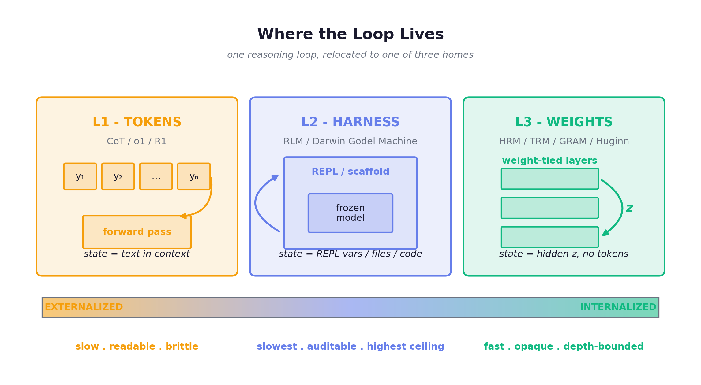
Here is the frame for everything that follows. Strip away the marketing and every method that makes an LLM stronger at inference does the identical thing: runs some loop a few more rounds before committing to an answer. Chain-of-Thought runs it. o1 and R1 run it. An agent scaffold that retries runs it. A recurrent-depth network runs it. They differ on exactly one design decision: where the loop runs, and where the loop’s state is stored while it runs. There are three positions.
L1, externalized to tokens. The loop carrier is the output token sequence; the state is the generated text sitting in the context window; the same forward pass emits tokens one at a time and feeds them back. This is CoT, o1, DeepSeek-R1. It is explicit, readable, and rewardable by RLVR, but slow (every step is a serial forward pass), brittle (one wrong sampled token cascades downstream), and data-expensive (you generally need step-by-step supervision or RL to teach it). The HRM camp calls CoT a crutch for exactly this reason.
L2, externalized to a harness. The loop carrier is outer code: an orchestration scaffold, an environment, a REPL. The state lives in REPL variables, files, or the evolving scaffold code itself. The model is frozen; a shell wraps it and, in the strongest version, rewrites itself. RLM is recursion-as-inference (it calls itself, depth 0 to 3, to chew through 10M+ tokens of context without rewriting itself). The Darwin Gödel Machine is recursion-as-self-modification (it edits its own tools and prompts, validated by benchmark fitness, never touching the kernel weights). Both are L2 but they are not the same thing; do not conflate them. Adaptation here is a slow analyze to rewrite to re-analyze cycle; the ceiling on expressivity is enormous and the trace is auditable, but every adaptation is a full re-run.
L3, internalized into weights. The loop carrier is latent-state recursion inside the network, along the depth axis. The state is a hidden vector that is never decoded and consumes no tokens. Shared weights are applied repeatedly. This is HRM, TRM, GRAM, HRM-Text, and the recurrent-depth / Huginn line. Adaptation happens within a single forward pass: you deepen compute on demand. It is strikingly data-efficient. The costs: training stability is genuinely hard, and you lose the readable chain, so it is far less interpretable.
| L1: tokens | L2: harness | L3: weights | |
|---|---|---|---|
| Loop carrier | output token sequence | outer code / scaffold | latent recursion along depth |
| State lives in | generated text in context | REPL vars / files / code | hidden state (no tokens) |
| Who changes it | the model, one token at a time | the scaffold (re-runs / rewrites) | weight-tied block, applied again |
| Adaptation speed | slow (serial passes) | slowest (re-run per turn) | fast (one forward pass) |
| Expressivity ceiling | medium | highest (10M+ tokens, self-edit) | medium, depth-bounded |
| Interpretability | high (readable chain) | high (auditable trace) | low (black box) |
| Exemplars | CoT, o1, R1 | RLM, Darwin Gödel Machine | HRM, TRM, GRAM, Huginn |
The same spectrum shows up again when you ask how to spend extra test-time compute. There is no single dial; there are four axes, and each one lands on a position above:
- Token axis. Unroll a longer CoT. Each extra token is roughly one more pass through the whole network. That is L1.
- Depth axis. Take more recursion steps, raise the ACT budget. HRM trains at a recursion budget of yet still gains accuracy when you push it to 16 at inference, with no retraining. That is L3.
- Width axis. Run several latent trajectories in parallel and select the best. GRAM with trajectories at 16 steps hits 97.0% on Sudoku-Extreme, beating a deterministic baseline run out to 320 steps at 90.5%. Also L3.
- Orchestration axis. More REPL rounds, deeper symbolic recursion. Highest ceiling, but every round restarts the system. That is L2.
Depth and width turn inside one forward pass, and width parallelizes; the orchestration knob re-runs the whole system on every turn. Marginal returns differ sharply by task. Depth, not width, is the decisive variable on Sudoku-Extreme, where adding parameters barely moves the needle.
This is also the trap the whole post is built to disarm. RLM and HRM are both sold as recursive, and the word does real work in both, but the recursion lives in completely different places. RLM recurses at the code-orchestration layer (L2); HRM recurses in network depth (L3). The point of the L1/L2/L3 spectrum is precisely to pull apart that ambiguity in the word recursion, because two systems can share a buzzword and share almost nothing mechanically.
Same loop, three places to put it, schematically.
       # L1: externalize the loop into tokens (CoT / o1 / R1)
for _ in range(N):                            # N serial forward passes
    toks += model.generate_one_step(toks)     # state = text in the context

# L2: externalize the loop into a harness (RLM / Darwin Godel Machine)
state = {}
for _ in range(N):                            # each turn re-runs the system
    state = harness.step(frozen_model, state) # state = REPL vars / files / code

# L3: internalize the loop into the weights (HRM / TRM / GRAM / Huginn)
z = init(x)
for _ in range(N):                            # all inside ONE forward pass
    z = f_theta(z, x)                         # state = hidden vector, never decoded
Three loops, three homes. Across this post I will place a bet I have to earn: under ARC-AGI-3’s step-scored, interaction-efficiency rule, the loop wants to live in the weights, because every externalized re-run burns scored steps, while a latent loop deepens for free. But that is the where, and the where is only half the title’s question. A loop runs over something, and before I argue about its address I owe you an account of its contents: what actually belongs in the kernel. So I am answering the what first. The next two chapters are about the substance of the kernel: the reasoning primitives a policy composes, and why composition, not the loop machinery, is where imitation breaks. Only after that do I come back to the how, how you put a loop in the weights at all, and earn the bet.
2. The Kernel Is Primitives
A model can hold every reasoning move there is and still fail the task, because possessing the moves was never the hard part. Chaining them into one it has never seen was.
Chapter 1 settled where a loop can live: in the tokens (L1), in the harness (L2), or in the weights (L3). Every way to make a model think harder reduces to running some loop a few more times before answering, and the only free choice is its address. But that answers HOW you relocate a loop, not WHAT the loop is chewing on. Relocate it onto what? If the kernel is the thing worth internalizing, we still owe the title a literal answer: what is the kernel made of?
Not facts. Facts belong in the shell, exact, unbounded, cloneable, better left in context or a tool catalog. The kernel is a small set of atomic reasoning primitives plus the control logic that coordinates them. A reasoning primitive is an atomic cognitive operation a model fires mid-task, between input and answer: not a fact it looks up but a move it makes. Here is the working register I keep, deliberately mixing toy games with real long-horizon decision work to make a point. Those “serious” tasks are not a different species, they are these same primitives composed over a longer horizon:
| Primitive | Atomic operation | Where it fires |
|---|---|---|
| Expected-value calculation | weigh outcomes by probability, pick the best bet | poker; pricing an insurance policy in underwriting |
| Case-by-case analysis | split the world into exhaustive cases, resolve each | logic-grid puzzles; claims adjudication across exclusion clauses |
| Backtracking | detect a dead end, unwind, try another branch | maze/Sudoku solving; diligence when a thread of evidence collapses |
| Sub-goaling | decompose a goal into ordered sub-goals | game planning; staging a multi-quarter deal |
| Verification | check a candidate answer before committing | proof-checking; reconciling figures against source documents |
| Deduction / abduction | derive entailments; infer the best explanation | rule inference; root-causing a fraud signal |
| Theory-of-mind | model another agent’s hidden state and intent | negotiation; counterparty risk in diligence |
Underwriting, diligence, claims, the things people call “judgment,” are not magic. They are this register, fired in long chains, under uncertainty, over many steps. That is the whole bet of the kernel: get these few operations and the composing control over them into the weights, and the long-horizon tasks follow.
Two grains, three layers
At the bottom are the Elements: the five fluid-intelligence (Gf) faculties, namely entity perception, concept abstraction, analogical reasoning, pattern/rule discovery, and memory revision. These are the co-active dimensions of on-the-fly reasoning, my decomposition grounded in Chollet’s On the Measure of Intelligence, which defines intelligence as skill-acquisition efficiency on genuinely novel tasks. Faculties are not a literal checklist; every concrete move blends several. One level up are the Bricks: the concrete operations in the table above, each exercising some mix of faculties. And one level above that is the Architecture: how bricks get assembled for a task never seen before, h = g∘f.
The essence lives at the top. A building is not its bricks; it is the way they are put together. Two models can hold an identical set of bricks and differ entirely in what they can build, because the capability that matters is the assembly, not the inventory.
The seam inside the bricks: content vs control
Look closely at the Bricks layer and a seam appears. Some bricks produce the answer: expected-value calculation, case analysis, deduction, abduction, theory-of-mind. Call these content bricks. Others do not produce the answer at all; they steer the search over the composition tree, by backtracking, sub-goaling, verification, backward-chaining. Call these control bricks. They are meta-bricks: bricks that assemble other bricks. Sub-goaling is decomposition, the inverse of g∘f. Backtracking is a control structure over the tree of partial compositions. So the control bricks sit closest to the Architecture layer. They are composition, expressed as operations.
This list is not arbitrary. It overlaps exactly the cognitive behaviors of self-improving reasoners catalogued by Gandhi et al.: backtracking, sub-goaling, verification, backward-chaining. And backtracking in particular is the kind of habit R1 was observed to grow on its own.
And here is the bridge I want planted, because it is the load-bearing idea of this whole post. The control logic that coordinates the primitives, the loop that proposes a composition, checks it, backtracks, decomposes, tries again, is a loop. It is the same kind of object Chapter 1 was relocating across L1/L2/L3. “Internalize the loop” and “internalize the composing control over primitives” are not two projects. They are the same kernel seen from two sides: the loop the rest of this post tries to push into the weights IS the control over primitives. Keep that equation in hand.
Composition, not possession, and why imitation can’t buy it
Now the crux. The bottleneck to capability is not holding the primitives. It is composing them: chaining f∘g into a procedure the model was never shown composed. Possession is cheap. Composition is the wall. And two negative results say plainly that imitation cannot climb it.
Faith and Fate (Dziri et al., 2023) probed transformers on multi-step compositional tasks (multi-digit multiplication, Einstein/Zebra-style logic-grid puzzles, a classic dynamic-programming problem) and found they do not execute the composition. They reduce it to linearized subgraph matching: pattern-completing memorized sub-templates of the computation graph instead of running the algorithm. They cheat. And because they cheat, accuracy decays as task complexity grows, because the memorized templates run out.
Skill-Mix (Yu et al., 2024) shows the same wall from the generative side. Pick a random subset of k skills plus a random topic, ask for a short text using all k. Single-skill recall is near-ceiling. But combining skills the model never saw combined collapses fast: weaker models struggle to combine even 3 skills, while GPT-4 holds reasonable performance at k=5, suggestive of going beyond stochastic-parrot behavior. The gap between “has the skills” and “can combine the skills” is the entire finding.
One honesty note: Faith and Fate documents that imitation-trained transformers don’t compose. It does not say “therefore RL.” That second step (SFT cannot compose, so reach for RL) is my takeaway, not theirs. Chapter 3 earns it.
Why imitation is structurally doomed here is just counting. The number of k-skill combinations grows like N^k, so any finite training corpus covers a vanishing fraction of the compositions the world will ask for. The model must generalize the assembly, because it can never have seen it. This snippet makes the blow-up concrete:
       from math import comb
N, corpus = 50, 100_000          # 50 skills; a generous SFT corpus of combos
for k in range(1, 6):
    space   = comb(N, k)         # distinct k-skill subsets
    covered = min(corpus, space) / space
    print(k, space, f'{covered:.1%} of combinations seen in training')
# k=1: 100% seen -> single-skill recall is trivial
# k=3: 19,600 triples < corpus -> 100% coverable, so still memorizable
# k=5: ~5% seen  -> must generalize; weak models collapse here
# The combinatorial blow-up is exactly why composition can't be bought with data.
Possession scales with data; composition does not, because the space of compositions outruns any corpus. So if SFT memorizes compositions and cannot generate them, what training signal actually composes primitives instead of recalling them? Chapter 3 names it, and it is not more imitation. It is RL under environmental demand: the one signal that learns to assemble bricks rather than file them.
3. Growing the Kernel with RL
Train a four-billion-parameter model to play poker with no arithmetic anywhere in the game, and it gets measurably better at math. That is what composition transferring across domains looks like.
Chapter 2 ended on a deflating result: imitation does not learn to compose, it learns to look like it composes. A transformer trained on demonstrations solves multi-step tasks by what Faith and Fate calls linearized subgraph matching, pattern-completing memorized sub-templates of the computation graph instead of running the computation, so accuracy decays as the chain gets deeper. Skill-Mix shows the same wall from the generative side: single-skill recall sits near ceiling, but ask for a short text using k skills never seen combined and weak models struggle to combine even three while GPT-4 still holds at k=5. SFT memorizes compositions and shatters out of distribution. So if the kernel is primitives plus the control logic that chains them, and imitation cannot grow the chaining, what can?
My answer is RL, and the cleanest demonstration is deliberately stripped of everything except composition. In From f(x) and g(x) to f(g(x)), Yuan et al. build a synthetic string-transformation framework: teach a model the atomic functions f and g, then ask whether it can produce the unseen composition h(x) = g(f(x)). RL learns the composition, generalizes to chains of more than two functions it never saw in training, and the compositional habit transfers to fresh tasks, needing only that the new task’s atomic skills are already known. SFT on the identical data yields none of this. Same corpus, same atoms; one method memorizes, the other synthesizes. I keep this calibrated: it is a synthetic toy, not ARC and not games, and the paper reports directions rather than headline percentages. But the direction is unambiguous and it is the whole thesis in miniature.
That looks like a clean toy result until you watch it reappear with a binding prerequisite in a real-world setting. Atomic to Composite decomposes complementary reasoning into two atomic skills: parametric reasoning over facts frozen in the weights, and contextual reasoning over novel in-context information, on a controlled synthetic-biography set. SFT a model directly on the composite task and you get the SFT Generalization Paradox: about 90% in-distribution on seen facts, collapsing to roughly 18% out-of-distribution on novel facts and paths. It memorized the joint, it never learned to integrate. RL then synthesizes the generalizing composition, but only if the base model has already mastered the atoms via SFT. RL alone on the composite task does not fix the collapse. Both the synthetic and the real-world line converge on the same recipe: Stage 1, SFT the atomic skills until mastered; Stage 2, RL the composite tasks. Atomic mastery first is not an ingredient you can skip. It is a precondition.
Here is that two-stage recipe, written so the prerequisite is an assertion you cannot quietly skip.
# Stage 1 — SFT each ATOMIC skill until mastered (the binding prerequisite).
for skill in atomic_skills: # e.g. f, g (or parametric- vs contextual-reasoning)
sft(model, data=demos_of(skill)) # imitation is fine for possession
assert all(mastered(model, s) for s in atomic_skills) # skip this and RL only 'amplifies'
# Stage 2 — RL on COMPOSITE tasks; reward only the final verifiable outcome.
# SFT on the identical composite data yields none of the generalization below.
for task in composite_tasks: # demands h = g(f(x)), depth > anything shown
traj = model.rollout(task)
reward = verify(traj.answer, task) # sparse, outcome-level
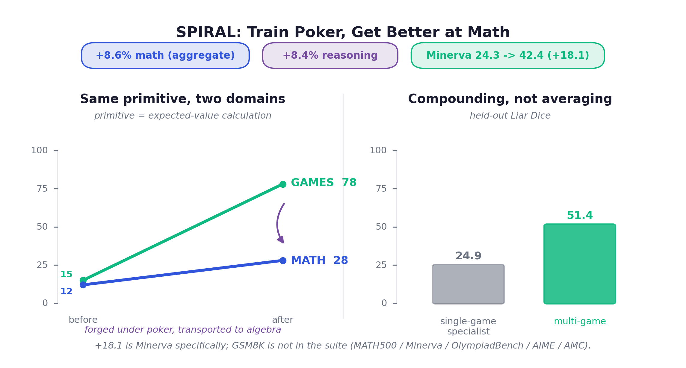
rl_update(model, traj, reward) # this is what learns to COMPOSE, not memorizeIf those two are the controlled proof, SPIRAL is the dramatic one. Liu et al. run self-play RL on multi-turn zero-sum games (TicTacToe, Kuhn Poker, Simple Negotiation) with role-conditioned advantage estimation. Self-play on a single game, Kuhn Poker on Qwen3-4B-Base, with zero math data anywhere, lifts math by +8.6% and general reasoning by +8.4% in aggregate. Drilling into one benchmark, Minerva Math goes 24.3% to 42.4%, a gain of 18.1 points. To be precise: the +18.1 is Minerva specifically, not the aggregate, and GSM8K is not in this paper. Its math suite is MATH500, Minerva, OlympiadBench, AIME and AMC. The mechanism is visible in the primitive itself. SPIRAL tracks expected-value calculation: inside the games it rises from 15% to 78%, and in the math domain from 12% to 28%. The same operation, forged under poker, transported to algebra. And the primitives compound rather than average: train across multiple games and on held-out Liar’s Dice the single-game specialists hit 24.9% while the multi-game model hits 51.4%.
Step back and the lever becomes clear. In every one of these results, a primitive, especially a control brick, appears in the policy only when an environment demands it. Dead-ends with verifiable failure breed backtracking; a long horizon breeds sub-goaling; a betting game with hidden information breeds expected-value calculation. Possession is cheap. The model can hold every primitive and still never chain them, because chaining is not summoned by having the parts. It is summoned by a task that cannot be solved without the chain. Which means the object you should be scaling is not the policy. It is the environment, its rule-set, and the variety of compositions it forces. This is the WHAT-grows-and-HOW answer the title of this part promised: the kernel is a compositional capability, and it grows under demand.
Now the counterweight, because the calibrated claim is narrower than the slogan. Cross-domain RL transfer is real but it is neither free nor universal. Sharpening a policy on one distribution can erode others. The generalization tax is a genuine cost, not a footnote, so transfer is a measured tendency in the settings studied, not a guaranteed Pareto win. The atomic-mastery prerequisite is binding: skip Stage 1 and RL only amplifies what is already there rather than synthesizing anything new. And most of these composition magnitudes are qualitative or synthetic; outside the regimes where they were measured, only the direction is a safe claim, never the number. My honest version of the thesis: RL composes primitives and the composition transfers, under a prerequisite, within studied regimes, possibly at a cost to other distributions.
So RL grows the compositions. But growing them leaves one question untouched: where does the composed control loop physically live? In everything above it is bought one of two ways, paid for in chain-of-thought tokens, each token roughly one more pass through the network, or bolted on with a harness that re-runs the scaffold every turn. Notice the bridge: the control logic that coordinates the primitives (backtracking, sub-goaling, verification) is itself a loop. Backtracking is a control structure over the composition tree; sub-goaling is decomposition, the inverse of g∘f. To internalize the composing control over primitives is to internalize a loop. The rest of this post asks whether that loop can instead live in the weights, and it starts with the most basic obstacle: why a fixed-depth transformer cannot simply choose to think longer.
4. The Fixed-Depth Wall
A transformer gets exactly as many sequential reasoning steps as it has layers, and not one step more, however hard the problem in front of it.
Chapter 1 laid out the three places an adaptive loop can live (in the tokens, in an outer harness, or inside the weights), and before we can argue about which one to internalize, we need to understand the wall that forces the choice.
That wall is depth. So let me separate three things that get conflated constantly.
Width is the per-step parallel bandwidth: hidden size, number of heads, FFN dimension. It is the highway lane count. Depth is the number of stacked, serial, mutually dependent nonlinear transforms a value passes through before it becomes an output. It is the number of traffic lights you must clear in order. Effective computational depth is the honest version of depth: the count of serial steps the network actually executes before emitting an answer, which for a standard transformer is at best its layer count and in practice less, because vanishing gradients keep deeper-than-necessary stacks from training cleanly.
Adding lanes never helps you clear twenty lights in sequence. Many reasoning tasks are intrinsically serial algorithms: backtracking, constraint propagation, any state where step has to wait for the result of step . Widening the pipeline cannot compress a ten-step serial dependency into fewer steps, because the dependency is the point.
The TC⁰ ceiling
A fixed-depth, per-layer-parallel transformer applies a constant number of serial transformations per output, no matter how difficult the input. That places a single forward pass in a shallow parallel circuit class, roughly (constant-depth, polynomial-size, threshold-gate circuits), and in more restricted settings . The chapter I’m drawing from states the inclusion chain . I want to be careful here: this is an intuition-level argument, not a tight proven theorem about transformers, and I am not going to present as an exact bound. But the direction is right. Problems believed to need non-constant serial iteration sit above , so they are inexpressible in one fixed-depth forward pass. And crucially, adding parameters does not help, because parameters buy width and memory, not the serial-depth dimension.
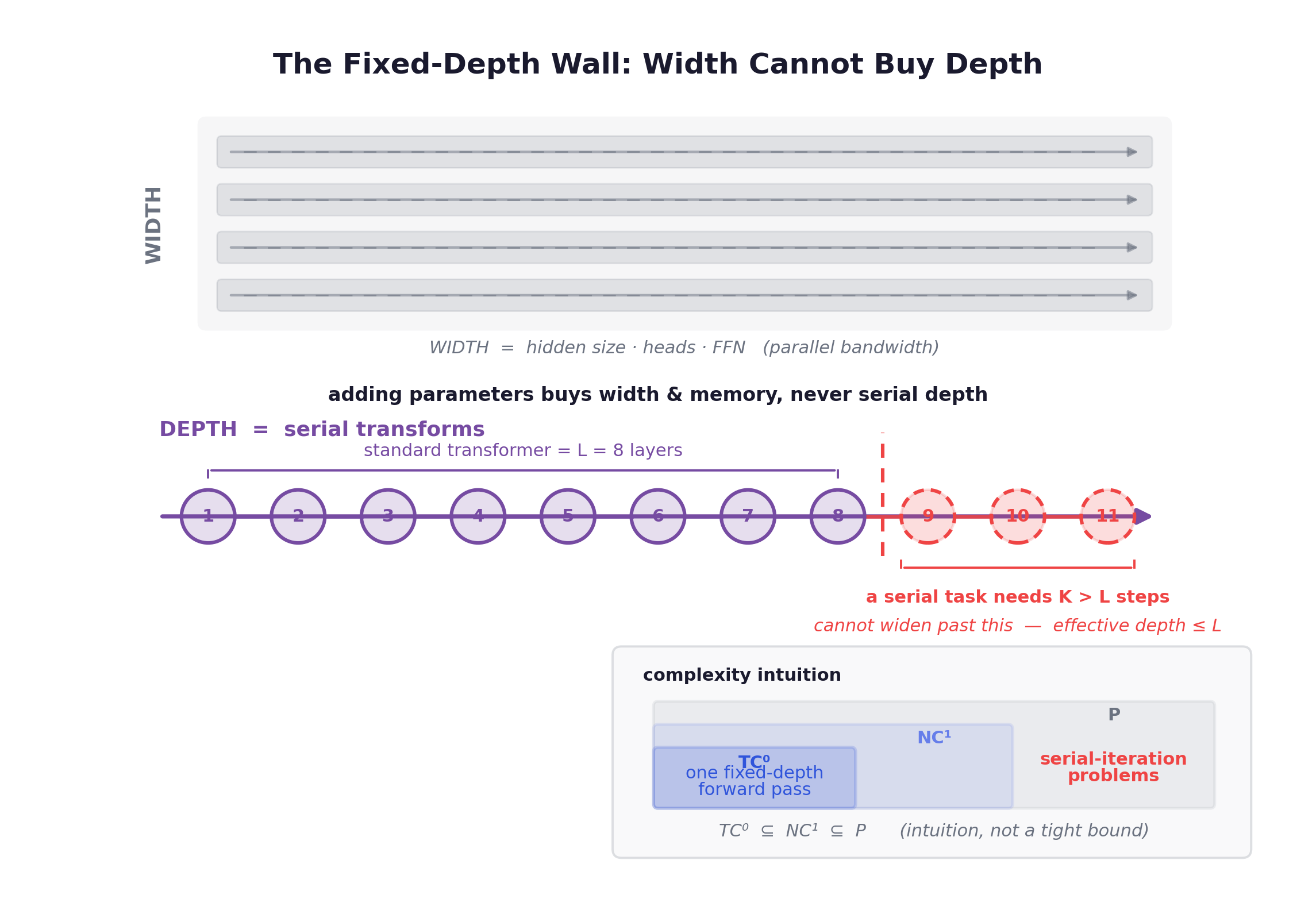
This is the precise sense in which a fixed-depth feedforward transformer is not Turing-complete. It is missing an axis, not just capacity.
The cleanest empirical demonstration comes from the Hierarchical Reasoning Model. On Sudoku-Extreme they fixed an 8-layer transformer and scaled parameters across 27M → 54M → 109M → 218M → 436M → 872M. Accuracy was essentially flat the whole way up. As HRM puts it, increasing a transformer’s width yields no performance gain, while increasing depth is critical. When they instead fixed hidden size 512 and scaled computed depth from 8 toward 512, depth helped, though the standard architecture saturated quickly, which is a separate problem I’ll come back to in the next chapters. The headline contrast: CoT-class SOTA models score 0% on Sudoku-Extreme and 30×30 Maze-Hard, while a 27M-parameter HRM trained on only 1000 samples, with no pretraining and no CoT, gets near-perfect accuracy.
Chain-of-thought is depth, borrowed from the token axis
So how do today’s reasoning models get away with fixed depth? They cheat, gracefully, by spending the token axis.
Chain-of-thought works because every generated token re-runs the entire network once. Emitting more intermediate tokens trades output length for additional serial compute. Formally, the model computes and samples , then re-embeds and feeds it back. Each token is one more serial step. This is the o1 / DeepSeek-R1 paradigm, and it genuinely raises effective depth. It is not magic; it is just depth externalized onto the output sequence.
But this is the L1 workaround, and it carries four costs at once. It is brittle: the reasoning state is serialized into a text chain with no differentiable error-correcting loop, so one bad sampled token cascades. It is slow: thinking tokens require forward passes that must run serially, so latency grows linearly with reasoning length. It is data-hungry: learning to write step-by-step generally needs large CoT supervision or RL. And it is token-level, which is the most insidious. A token carries only bits, while the hidden state being squeezed through that softmax is a continuous vector of thousands of dimensions. Forcing each reasoning step through a single discrete word is a lossy projection. This is the HRM camp’s “language is a tool for communication, not the substrate of thought” framing: for reasoning, language is an output format, not a computation medium.
If the problem with CoT is that the inter-step state has to pass through a discrete softmax bottleneck, the obvious alternative is to keep that state continuous and add the serial steps inside the network instead. Here is the simplest possible internalized loop: one shared block applied K times to grow effective depth without adding a single parameter.
       import torch
import torch.nn as nn
from recursive_kit import make_net

class LoopedNet(nn.Module):
    """Apply ONE shared block n_loops times along depth.

    h^{(0)} = x
    h^{(t+1)} = f_theta(h^{(t)}, x),  t = 0 .. n_loops-1

    Every loop reuses the same parameters, so 'going deeper'
    is decoupled from 'adding parameters'.
    """
    def __init__(self, dim: int, seed: int = 0):
        super().__init__()
        self.dim = dim
        self.block = make_net(dim, seed)   # exactly one block

    def forward(self, x: torch.Tensor, n_loops: int) -> torch.Tensor:
        h = x
        for _ in range(n_loops):
            h = self.block(h, x)   # re-inject x so we never lose the problem
        return h

# Param count is independent of n_loops; n_loops=0 is the identity.
# Train with small n_loops, run larger n_loops at inference:
# the seed of length generalization — more loops = more serial compute.
The logic that gets us here is almost forced. If a serial problem needs more reasoning steps than you have layers, you have exactly two moves. You can add tokens, which is CoT, and you pay the four costs. Or, if you cannot or will not add tokens, the only remaining way to think longer is to add depth. And the cheapest way to add depth without exploding parameter count is to loop the same weights, exactly as LoopedNet does above: iterations of give effective depth while the parameter count stays fixed at one block’s worth.
That single idea, depth as a runtime quantity decoupled from parameters, is what the next chapter builds real architectures on, from the Universal and Looped Transformers to recurrent-depth latent reasoning.
5. The Recurrence Revival
The cure for a depth wall is not a taller stack of bricks. It is one brick you walk through over and over.
Chapter 4 showed that a bare looped block lifts effective depth without touching parameter count, and once you see that, a whole genealogy of architecture snaps into focus.
The enabling idea is older and more boring than it sounds: weight tying. A standard Transformer with layers learns independently parameterized blocks and runs each exactly once. Weight tying collapses that into a single shared block applied repeatedly along depth:
The hidden state is the inner state carried across iterations; is the original input, re-injected each loop so the block always knows what problem it is solving. The consequence is the whole point. Computational depth is now , but the parameter budget is one block’s worth, independent of . You decouple “going deeper” from “adding params.” The LoopedNet above makes this concrete: it holds exactly one shared block, and its parameter count is independent of n_loops, equal to a single block’s. That is the core weight-tying assertion stated as plainly as it can be.
The lineage
The Universal Transformer (Dehghani et al., 2018, the foundational systematization) folded the distinct layers into one shared block applied repeatedly. Its two contributions matter here. First, it injects a per-step timestep embedding so the shared block can distinguish which recurrence step it is on. A tied block applied five times needs to know whether it is on iteration 1 or iteration 5. Second, it adds ACT-style adaptive halting: each position emits a halting probability and freezes once a threshold is reached, so easy tokens stop early and hard tokens iterate longer. With recurrence plus dynamic halting, the Universal Transformer is proven Turing-complete given enough steps. HRM explicitly places itself in this same class. (The honesty caveat from the previous post applies: Turing-completeness here is an asymptotic, idealized claim requiring sufficient memory and time. It says nothing about sample efficiency or trainability, so do not conflate the entry ticket with actually winning the race.)
The Looped Transformer (Yang et al., 2023) reframed the same machinery as executing an iterative algorithm in latent space. Loop the shared block times, re-injecting each loop, and the loop count corresponds to algorithm iterations. Its signature result is length generalization: supervise with a small , and the model still solves harder instances at inference with . That is evidence it learned a reusable iterative rule rather than a fixed-depth lookup table. In GRAM’s controlled ablation the plain Looped Transformer is the simplest recursive backbone, a 7M-parameter model scoring 61.3 on Sudoku, before any deep supervision or hierarchical recursion is layered on. (Worth flagging: that 7M / 61.3 figure is a baseline within an ablation, not a standalone SOTA, and the length-generalization claim is for algorithmic tasks, not arbitrary natural-language reasoning.)
The most recent rung is recurrent-depth latent reasoning: Geiping et al., 2025, codenamed “Huginn.” Same recurrence , but now scaled at inference. The iteration count is the effective computational depth, and it can be dialed freely at test time, an axis orthogonal to adding parameters or data. The framing is sharp: language is a tool for communication, not the substrate of thought. Where Chain-of-Thought scales test-time compute by emitting more tokens, Huginn scales it inside the latent representation, no tokens spent.
The duality that makes it all work
Here is the crucial point, and it is what separates this lineage from a plain RNN. Because the same block is reused across steps, the number of recurrence steps is a runtime quantity, not a baked-in architectural constant. Train with steps, run with at inference, and you push more compute through the identical weights with zero retraining.
Two views of the same loop coincide:
| View | What the index means | What loops | Resulting object |
|---|---|---|---|
| Depth view | layer index | over depth | weight-shared deep net |
| Time view | time step | over a fixed input | RNN iterating in place |
The distinction from a classic RNN is worth being precise about. An RNN loops over time: each step consumes a new input token and advances a sequence. Recurrent-depth loops over depth, where the input is fixed, and each iteration is another serial nonlinear refinement of the same hidden state before any output is emitted. One walks forward through a sentence; the other thinks harder about a single position.
This is the cleanest realization of “internalize the loop” from the previous post. More compute means more iterations of one shared block. No extra parameters. No extra tokens. The adaptive budget lives entirely inside the weights, and the dial sits in your hand at inference time.
The forward pass below exposes loop count as a test-time argument and carries the inner state z across iterations; depth becomes a knob you turn after training, not a number you bake in.
       import torch
import torch.nn as nn
from recursive_kit import make_net

class RecurrentDepthNet(nn.Module):
    """One shared block iterated n_loops times along DEPTH.

    z^{(0)} = x
    z^{(t+1)} = f_theta(z^{(t)}, x),  re-inject x every step

    Param count is independent of n_loops: depth is decoupled from params.
    """
    def __init__(self, dim: int, seed: int = 0):
        super().__init__()
        self.block = make_net(dim, seed)        # exactly ONE block, tied

    def forward(self, x: torch.Tensor, n_loops: int) -> torch.Tensor:
        z = x                                   # inner state carried across iters
        for _ in range(n_loops):
            z = self.block(z, x)                # f_theta(z, x); x re-injected
        return z

net = RecurrentDepthNet(dim=256)
x = torch.randn(8, 256)
shallow = net(x, n_loops=4)     # train-time budget
deep    = net(x, n_loops=32)    # spend MORE test-time compute, SAME weights
# n_loops is a runtime dial: test-time depth scaling with zero new params.
The catch is that all iterations are constrained to the same function, which is why residual connections and normalization are non-negotiable for stable looping, and even those only push back the vanishing-gradient wall rather than remove it.
But the deeper problem is on the training side: if inference runs 32 loops, naive backprop through those iterations caches every intermediate state and pays memory. That is exactly the trap chapter 6 confronts, and the elegant equilibrium-based fix it offers.
6. Training a Loop Cheaply
Running the loop a hundred times is trivial; the trick is learning from it without storing a hundred copies of your activations.
Chapter 5 made depth a test-time dial: tie the weights, iterate the same block as many times as the input deserves, and you spend more compute on harder problems without growing the parameter count. That dial is free at inference. It is not free during training, and the cost is exactly what kept looped weights off the frontier for years.
The wall: BPTT is O(depth)
Backpropagation through time is unforgiving. If your forward pass iterates a block times, autograd has to keep every intermediate activation alive so the backward pass can chain through all of them. Memory scales as . Loop a 27M-parameter block a few hundred times and you are no longer training a small model. You are training the unrolled equivalent of a network hundreds of layers deep, and the activation tensors for that depth simply do not fit. This is the structural reason “just iterate more” was a forward-pass party trick and not a training recipe.
The escape is to stop thinking about the iterations at all. As the framing I keep coming back to puts it: do not think of recurrence as stacking many layers. Think of it as solving an equation.
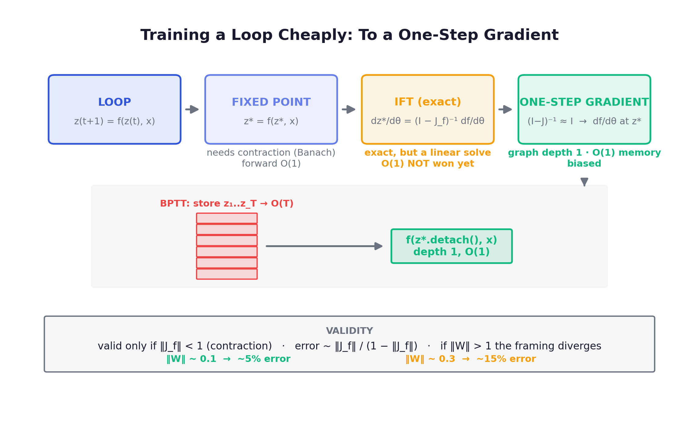
Reframe: the loop has a fixed point
Take a weight-tied update . If is a contraction in (Lipschitz constant below 1) the Banach fixed-point theorem guarantees the iteration converges to a unique equilibrium , exponentially fast. The Deep Equilibrium Model (Bai, Kolter and Koltun, NeurIPS 2019) makes this the whole point of the architecture: an “infinite-depth” weight-shared network is just a solver for that equilibrium. Depth stops being a hyperparameter you set and becomes the number of iterations needed to converge: implicit, and decided by the input. Easy inputs settle in a few steps, hard ones take more. That is the same adaptive-compute story from Chapter 5, now with a clean mathematical object underneath it.
The forward pass is unglamorous: iterate until the residual drops below a tolerance.
The exact gradient: implicit function theorem
The fixed point satisfies , where is implicitly a function of . Differentiate both sides with respect to and rearrange:
where is the Jacobian evaluated at . The gradient depends only on the fixed point and the local Jacobian there, not on the trajectory that reached it, not on how many iterations it took. Backward cost is decoupled from forward depth. You never unroll.
The catch is the term. The implicit function theorem hands you an exact gradient, but exact still means solving a linear system involving that matrix inverse on every backward pass. The O(1) memory win is not yet realized: IFT alone trades a tall activation stack for a linear solve.
The trick: Neumann series, truncated to one term
Expand the inverse as a Neumann (matrix geometric) series:
which converges precisely when is a contraction (spectral radius of below 1). Now truncate to the first term: . The gradient collapses to
This is the one-step gradient. Operationally it is almost embarrassingly simple: solve for under no_grad, detach it, then run exactly one more forward call that carries gradient. The computation graph is depth-1 regardless of whether the forward pass iterated a handful of times or ran all the way to its iteration cap. Memory drops from to . That single line, store nothing from the loop and backprop through only the last step, is what turns a test-time dial into a trainable architecture.
The DEQ forward plus one-step gradient:
A no-grad fixed-point solve followed by a single gradient-carrying step.
       import torch

def fixed_point_forward(f, z0, x, max_iter=300, tol=1e-7):
    """No-grad iteration z = f(z, x) until ||z_next - z|| < tol. Memory is O(1)."""
    with torch.no_grad():
        z, n_iter, residual = z0, 0, float("inf")
        for k in range(max_iter):
            z_next = f(z, x)
            residual = (z_next - z).norm().item()
            z, n_iter = z_next, k + 1
            if residual < tol:
                break
    return z, n_iter, residual

def deq_solve(f, z0, x, max_iter=300, tol=1e-7):
    """Solve to z* under no_grad, then take ONE gradient-carrying step.
    autograd here yields the Neumann first-term approx of (I - J_f)^{-1} df/dtheta."""
    z_no_grad, _, _ = fixed_point_forward(f, z0, x, max_iter=max_iter, tol=tol)
    z_star = f(z_no_grad.detach(), x)   # graph depth = 1, independent of iterations
    return z_star
How wrong is it, and when
Be honest: this is a biased approximation, not the exact IFT gradient. The sources mark it plainly so, but effective in practice. The error you pay for dropping the higher-order terms scales like , so the more strongly contractive the map, the cheaper the truncation. The intuition is clean: if the system has already converged, one more step barely moves , so the discarded terms contribute almost nothing.
A toy example makes this concrete with the contraction map . At spectral norm of around 0.1, the one-step gradient lands within roughly 5% relative error of full BPTT, with cosine similarity above 0.99. Push the spectral norm to 0.3 and the relative error grows to about 15%, matching the prediction.
| Spectral norm | 1-step relative error |
|---|---|
| ~0.1 | ~5% |
| ~0.3 | ~15% |
These numbers belong to the toy map, not to any production model, so do not read them as accuracy claims about real recurrent-depth systems. The load-bearing caveat is the validity condition: the one-step gradient is justified only when the forward pass genuinely converges to a fixed point, which requires a contraction. If the spectral norm exceeds 1, the forward iteration diverges and the whole equilibrium framing, along with its gradient, falls apart. This fixed-point assumption is exactly what chapter 8 challenges: TRM shows HRM never truly converges, and full-segment backprop beats the one-step gradient anyway. Hold onto that assumption: chapter 8 challenges it directly, showing that the loop HRM trains this way never actually converges and that backpropagating the full segment beats the one-step gradient outright.
How many steps? A learned halting head
The fixed-point view answers “how do I train a deep loop cheaply.” It leaves open “how many iterations should this input get.” The oldest answer is Adaptive Computation Time (Graves, 2016): attach a halting unit that emits a scalar at each thinking step, accumulate those probabilities, and stop at the first step where the cumulative sum crosses . The output is the halting-weighted average of per-step outputs, with the last step absorbing the residual, which keeps the output differentiable in even though the step count is discrete. A ponder cost penalizes thinking longer, so task loss and ponder cost play tug-of-war and settle on just-enough depth. (PonderNet, Banino et al. 2021, recasts this as a halting distribution with a KL prior, more stable, though the sources give no head-to-head number.) ACT is the seed of input-adaptive depth, and the question it opens, who decides when to stop and how, is Gap A that the later chapters return to.
A minimal ACT-style halting loop that accumulates halting mass until threshold:
       import torch

def act_halt(steps, halt_head, x, eps=1e-2, max_steps=16):
    """Iterate 'thinking' steps; stop when cumulative halting prob crosses 1 - eps."""
    h = x
    cum_p, out = 0.0, 0.0
    for n in range(max_steps):
        h = steps(h, x)
        p = torch.sigmoid(halt_head(h)).clamp(eps, 1 - eps)
        remainder = 1.0 - cum_p
        is_last = bool(cum_p + p >= 1 - eps) or (n == max_steps - 1)
        weight = remainder if is_last else p   # last step takes the residual mass
        out = out + weight * h
        cum_p = cum_p + p
        if is_last:
            return out, n + 1
The equilibrium reframe plus the one-step gradient is the machinery that makes all of Part III possible, and the first model to ride it straight through a benchmark nobody could touch is HRM, which breaks ARC-style reasoning with just 27M parameters.
7. HRM: Altitude Emerges
A 27M-parameter network with no pretraining and no chain-of-thought out-reasons models with orders of magnitude more parameters on the exact puzzles that scale forgot.
Chapter 6 gave us the two ingredients that make latent recursion trainable at all: the one-step gradient that buys O(1) memory, and ACT halting that buys adaptive compute. The Hierarchical Reasoning Model assembles them into the canonical reference point for the whole post: an adaptive reasoning loop that lives entirely inside the weights, halting by a policy the model learned for itself. And buried in its analysis is the mechanistic seed of the claim I want to land by the end, that representational altitude is not configured, it emerges.
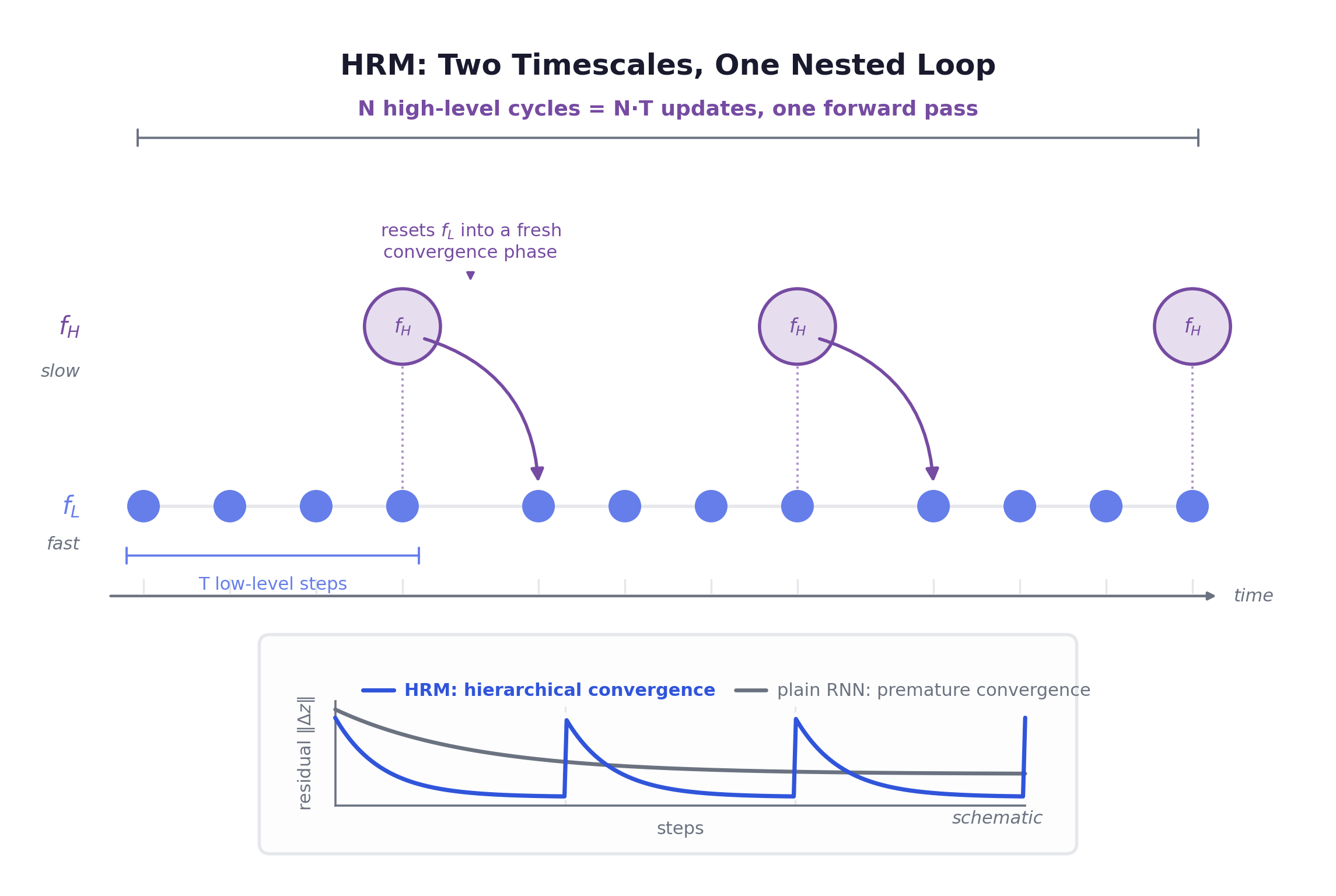
Two timescales, one nested loop
HRM couples two recurrent modules that are structurally the same encoder-only Transformer block (RoPE, GLU, RMSNorm, Post-Norm, no bias) but run on different clocks. The low-level module updates every timestep: fast, dense, detail. The high-level module updates only once every low-level steps: slow, abstract, planning. Within a cycle sees a fixed as its target and iterates toward it; then absorbs ‘s final state and advances once. Inputs are merged by plain element-wise addition. Run high-level cycles of steps each and you get total updates in a single forward pass.
The reason this is more than a deep RNN is hierarchical convergence. A plain recurrent net reaches a fixed point in roughly steps and then dies. Update magnitudes decay, and extra steps compute nothing. That is premature convergence, and it caps a recurrent net’s effective depth no matter how long you unroll it. HRM dodges it by making the convergence local and repeated: settles into an equilibrium that depends on the current , then updates once, which resets into a fresh context and a brand-new convergence phase. Chaining individually-stable sub-computations lifts effective computational depth to about while the forward residual stays high, because ‘s residual spikes again every cycle instead of collapsing to zero. You get the depth of a very deep network without the gradient pathologies of unrolling one.
The training recipe, end to end
The forward pass uses the one-step gradient from chapter 6. The first steps run under no_grad: no graph, no BPTT, constant memory. Only the final pair carries gradient, which is exactly the Neumann-series truncation : treat every intermediate state as constant, let credit flow only output head → final → final → input.
The HRM single-segment forward runs N·T steps under no_grad, then exactly one grad-bearing fL+fH:
       def hrm_inner(fL, fH, zL, zH, x, N, T):
    # First N*T - 1 steps: no gradient, no graph, O(1) memory (no BPTT).
    with torch.no_grad():
        for i in range(N * T - 1):
            zL = fL(zL, zH, x)              # fast / detail: every step
            if (i + 1) % T == 0:
                zH = fH(zH, zL)            # slow / abstract: every T steps, resets fL
    # Final step WITH gradient — the 1-step approximation: (I - J)^{-1} ~ I.
    zL = fL(zL, zH, x)                      # exactly 1 fL +
    zH = fH(zH, zL)                         # exactly 1 fH carry gradient
    return zL, zH
Over that inner loop sits an outer one: deep supervision. The same example is run through HRM as a sequence of segments. Each segment starts from the previous segment’s latent state, computes a loss, and updates parameters, but the state is detach()’d at the boundary so gradients never cross between segments. The detach is itself a one-step approximation of the recursive supervision process, and empirically it regularizes better than Jacobian-based alternatives while giving more frequent feedback.
Deep supervision runs M segments over one example, detaching latent state so gradients never cross a boundary:
       def deep_supervision(segment_fn, state0, x, segments):
    outs, state = [], state0
    for _ in range(segments):
        state = _detach_state(state)        # cut the graph between segments
        state, out = segment_fn(state, x)   # one HRM forward pass
        outs.append(out)
    return outs

def _detach_state(state):
    if torch.is_tensor(state):
        return state.detach()
    if isinstance(state, (tuple, list)):    # HRM state is (zL, zH)
        return type(state)(_detach_state(s) for s in state)
    return state
How many segments? That is what the ACT Q-head decides. A two-action head reads and predicts over an episodic MDP: halt to end with reward , continue for another segment. No replay buffer, no target network; stability comes from Post-Norm, RMSNorm and AdamW. The payoff is free inference-time scaling: train with , then raise it to at inference and accuracy still climbs, with no retraining and no architecture change.
The numbers
Per task: ~27M parameters, ~1000 input-output examples, trained from random init, no pretraining, no CoT supervision. On ARC-AGI-1 that gives 40.3%, against o3-mini-high at 34.5%, Claude 3.7 with 8K context at 21.2%, and DeepSeek R1 at 15.8%, all models with orders of magnitude more parameters and context. On the harder ARC-AGI-2 it scores 5.0% (o3-mini-high 3.0%, others ~0–1.3%). On Sudoku-Extreme (9×9) it hits 55.0% and on Maze-Hard (30×30) 74.5%, both where direct-prediction and CoT models score essentially 0%. An 8-layer Transformer in the same setup gets 0% at 1000 examples, and only 16.9% on Sudoku even with the full 3,831,994-example dataset.
| Benchmark | HRM | o3-mini-high | Claude 3.7 (8K) | Direct-pred (8L) |
|---|---|---|---|---|
| ARC-AGI-1 | 40.3% | 34.5% | 21.2% | 0% @1k |
| ARC-AGI-2 | 5.0% | 3.0% | ~0–1.3% | — |
| Sudoku-Extreme | 55.0% | ~0% | ~0% | 16.9% (full data) |
| Maze-Hard | 74.5% | 0% | 0% | — |
The intermediate-trajectory visualizations read like a world-model search in miniature: on mazes the latent state explores then prunes; on Sudoku it does DFS with backtracking; on ARC it hill-climbs toward the answer. Different algorithm per task family, chosen by the model. Suggestive, though the authors are explicit that what HRM internally implements is beyond their current scope.
Exploring then pruning, depth-first search with backtracking, hill-climbing toward a goal: these are exactly the kernel’s control primitives, the moves that steer a search rather than produce an answer. The reasoning-primitives work argued the hard, transferable thing to internalize is not the primitives but the control logic that composes them, and that imitation cannot install it. Here that control logic is, condensed into a latent loop and learned from a thousand examples. The H and L split even lines up with the content-versus-control seam from that argument: the slow planner steers the search while the fast worker executes the moves, control on top, content below. The composing loop the primitives literature could only grow with reinforcement learning is the same loop HRM bakes into recurrent depth.
The detail that matters most: altitude emerges
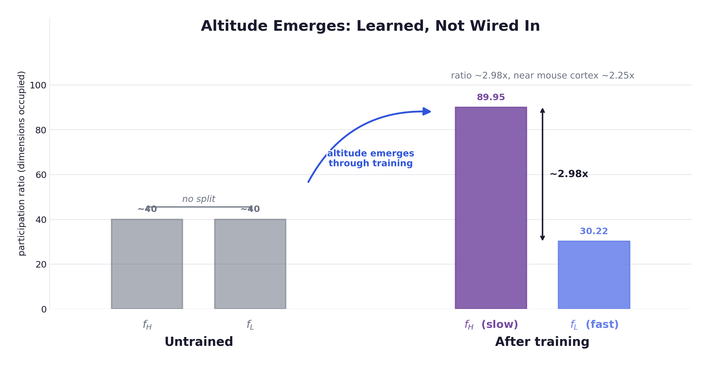
Measure the participation ratio, over the eigenvalues of each module’s trajectory covariance, a soft count of how many dimensions the representation actually uses. After training, sits at PR ≈ 89.95 and at PR ≈ 30.22, a ratio of ~2.98, strikingly close to the ~2.25 measured across mouse cortex. The slow module learned to occupy a far higher-dimensional, more abstract subspace than the fast one.
And it is learned, not built in. An untrained network shows both modules at PR ≈ 40 with no split at all; the hierarchy appears only through training, the opposite of the neural collapse seen in ordinary deep nets. Nobody assigned the role of “abstraction.” A higher representational altitude condensed in the slow recurrent module on its own. That is the mechanistic seed of altitude = depth, and I will cash it out in chapter 13.
Honest limits
HRM is offline, single-episode symbolic reasoning: one puzzle in, one grid out. There is no environment interaction, no cross-step world-model update, no reward-driven online adaptation. The Q-learning decides only how many segments to run, never how to act in a world. The paper does not touch ARC-AGI-3. ARC-AGI-2 at 5.0% is barely off the floor. The brain correspondence is correlational and explicitly not causal. The one-step gradient is exact only if truly reaches a fixed point with spectral norm of ; otherwise it is a biased approximation. And the setup leans task-specific (a per-task learnable token, ~1000 augmented variants, voting) in tension with ARC’s true few-shot spirit. HRM proves the loop can live in the weights; it does not yet prove that loop can live in a world.
All of which raises the obvious question that chapter 8 takes head-on: if a 27M network does this much, is HRM’s two-module, two-timescale, hierarchical-convergence machinery actually necessary, or is most of it scaffolding we can throw away?
8. TRM: Less Is More
Strip away the hierarchy, backprop through the whole loop on purpose, shrink it to seven million parameters, and watch it get better.
Chapter 7 laid out HRM’s full machinery: two timescales, hierarchical convergence, a one-step gradient justified by deep-equilibrium theory, ACT halting via Q-learning. It is a beautiful pile of moving parts. So I want to push on the uncomfortable question a team at Samsung SAIL Montréal asked. Which of these parts is actually load-bearing? They answered it by deleting most of them. The result is TRM (Tiny Recursive Model): a single tiny network with only 2 layers and 7M parameters that beats the 27M-parameter HRM on the same puzzles. Less is more, and the paper means it literally.
What survives the cut
TRM keeps exactly two ideas from HRM and throws out the rest. It keeps recursion, refining an answer over and over inside a single forward, and it keeps deep supervision, running the same example through up to N_sup=16 segments, detaching state between them. Those are the survivors. What it drops is everything that made HRM sound biological. The H/L hierarchy is gone. The two latent states z_H and z_L are no longer high-level planner and low-level executor; TRM re-reads them as a current answer y (decode z_H through the output head and you get an actual Sudoku board) and a latent reasoning feature z that does not decode to a valid solution but can be turned into one. So there is no hierarchy at all, just an input x, a proposed answer y, and a reasoning draft z. The model refines z, then uses z to update y. The ablation backs this exact framing: two features (y, z) score 87.4% on Sudoku-Extreme, multi-scale z (7 scales) drops to 77.6%, and a single z collapses to 71.9%. z is the chain-of-thought (“how I got here”); y is the answer (“what I last said”). Lose either and the model either forgets its reasoning or crowds it out.
The gradient is the whole point
The biggest cut is also the most surprising. HRM justified backpropagating only the last 2 steps by invoking DEQ and the implicit function theorem: assume the recursion reaches a fixed point, truncate the Neumann series to its first term, and you get O(1) memory and exactly 2 grad-bearing calls per segment. TRM throws the assumption out, because HRM never actually reaches a fixed point: its residual is nowhere near converged, so the justification was always a fiction. TRM instead backprops through the entire final segment, all n+1 net calls, not a constant 2.
The numbers settle the argument. One-step gradient (HRM-style) gives 56.5% on Sudoku-Extreme; full-segment backprop jumps to 87.4%. The authors even ran true fixed-point iteration with TorchDEQ, and it was slower AND worse. Converging to a fixed point is not just unnecessary, forcing it hurts. And the intermediate compromise (backprop only the last k=4 of n=6 steps) gave no improvement at all, only more complexity. It is all-or-nothing: the full segment, or you leave most of the accuracy on the floor.
There is a principled reason, and it tells you how much weight the math in chapter 6 can bear. A contraction map pins the Jacobian’s spectral norm below 1, which caps how much each step can transform its state, the opposite of the expressive range long-range reasoning needs. So the equilibrium machinery is not wrong; the architecture never needed it. The implicit function theorem bought a memory-saving training trick, valid only while the loop happens to converge, not the foundation the loop stands on. Treat chapter 6 as an elegant optimization, not the proof that latent loops are universally trainable.
| HRM (1-step / DEQ) | TRM (full-segment) | |
|---|---|---|
| grad-bearing net calls per segment | 2 (1 fL + 1 fH) | n+1 (n reasoning + 1 answer) |
| memory in segment | O(1) | O(n), can OOM at large n |
| networks | f_H + f_L (two) | one shared net |
| fixed-point assumption | yes (IFT/Neumann) | none |
| Sudoku-Extreme | 56.5% | 87.4% |
The TRM core (paper Figure 3); note the absence of any no_grad around the final segment. Every call in it gets a backward pass.
       def latent_recursion(net, x, y, z, n):
    # one full recursion process = n reasoning steps + 1 answer step
    for _ in range(n):
        z = net(x, y, z)   # refine reasoning z, conditioned on x (3 inputs)
    y = net(y, z)          # refine answer y from z, WITHOUT x (2 inputs)
    return y, z

def deep_recursion(net, x, y, z, n, T):
    # first T-1 segments: NO gradient, just push (y, z) toward the solution
    with torch.no_grad():
        for _ in range(T - 1):
            y, z = latent_recursion(net, x, y, z, n)
    # final segment carries gradients through ALL n+1 net calls.
    # Contrast chapter 7's HRM: there the whole inner loop sat under
    # torch.no_grad() and exactly 2 calls got gradients. Here: n+1.
    y, z = latent_recursion(net, x, y, z, n)
    return y, z
With the defaults n=6, T=3, the effective depth is , a 42-layer-deep computation from a 2-layer net, while only the last 7 calls (n+1) build a graph. The first T-1 segments under no_grad act as free residual, simulating an ultra-deep net without paying for its memory; the real credit assignment happens across the full final segment.
One shared net replaces HRM’s two: the only signal distinguishing the roles is whether x is summed in. net(x, y, z) is a reasoning step, net(y, z) is an answer step. Separating into f_H/f_L scores 82.4% versus 87.4% and doubles the parameters. And adding layers actively hurts: 4 layers gets 79.5% versus 2 layers at 87.4%. With ~1000 samples per task and no pretraining, capacity is the enemy; you want depth from recursion, not from width.
The lesson, stated plainly
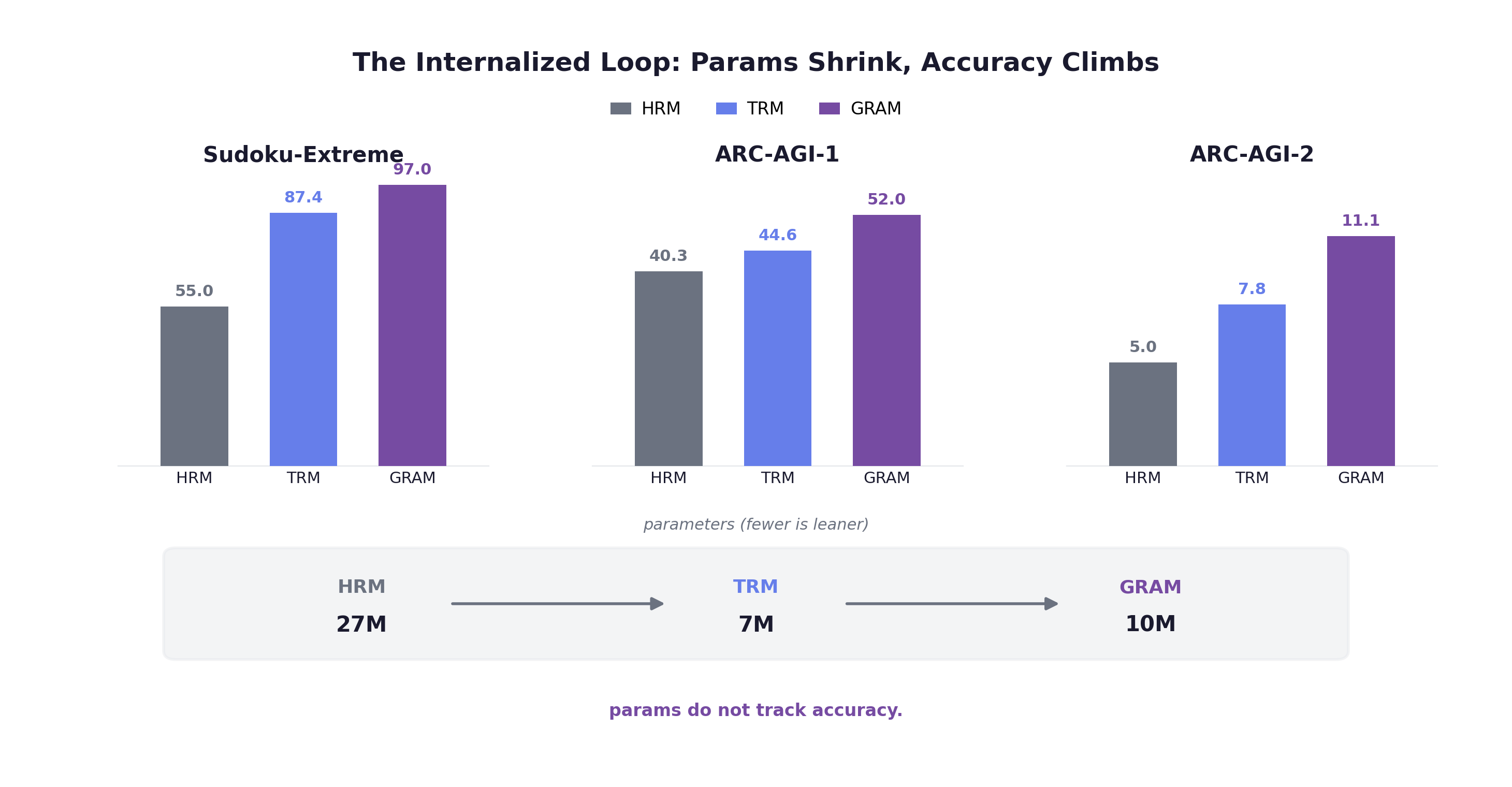
The load-bearing ingredients are recursive refinement and deep supervision, not the elaborate hierarchy, not the fixed-point story. An ARC Prize independent analysis of HRM (cited by TRM, not TRM’s own ablation) found deep supervision drove most of HRM’s gain, 19% to 39% on ARC-AGI, while the hierarchical recursion added only 35.7% to 39.0%. TRM takes that finding and runs: it is the minimal viable internalized loop. And it wins where the giants do not. Deepseek R1 (671B), o3-mini, and Claude 3.7 all score 0.0 on Sudoku-Extreme, while TRM hits 87.4% with its 5M MLP-Mixer variant (the 7M attention variant carries the Maze and ARC numbers, and even 7M is under 0.01% of R1’s params). On the headline benchmarks: Sudoku 55.0 to 87.4, Maze-Hard 74.5 to 85.3, ARC-AGI-1 40.3 to 44.6 (past o3-mini-high’s 34.5 and Gemini 2.5 Pro’s 37.0), ARC-AGI-2 5.0 to 7.8.
I want to be precise about scope, because the result is easy to oversell. These are small symbolic puzzles, ~1000 samples per task, no pretraining, test-time weights frozen, single deterministic answer. TRM is not a general language model, and the “no hierarchy” claim is a re-interpretation supported by ablations on these datasets, not a proof that hierarchy is meaningless everywhere. The paper offers no theory for why recursion beats a bigger net; the authors suspect overfitting and say so. But the engineering verdict is clean: a tiny recurrent core, supervised deeply, backpropagated fully, is enough to internalize a reasoning loop. What it still cannot do is say “I don’t know”. TRM commits to one answer and never measures its own confidence, which is exactly the gap GRAM closes by adding uncertainty.
9. GRAM: A Probabilistic Loop
A deterministic recursor locks onto its first guess and polishes it forever; fluid reasoning keeps several guesses on the table until the evidence picks the winner.
Chapter 8 gave us a minimal deterministic recursor: one latent state, refined in place until it settles. That model has a structural flaw that no amount of extra depth can fix. Given the same input and initialization, it traces exactly one latent trajectory and converges to exactly one answer. GRAM (Generative Recursive reAsoning Models, KAIST / Mila / NYU / Université de Montréal, 2026) is the fix. It turns that single-path loop into a generative one.
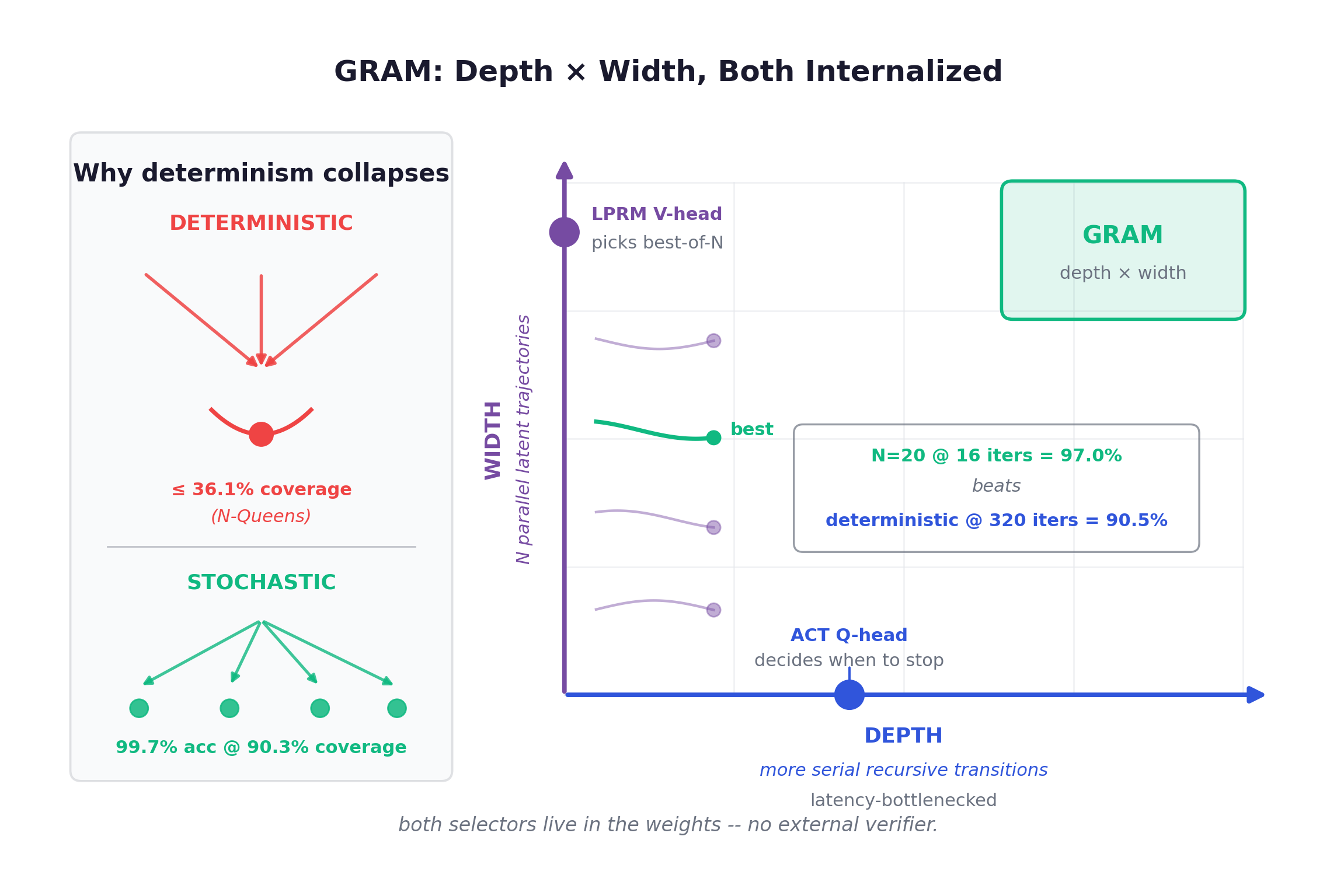
Why determinism collapses
A deterministic latent update is an attractor. Repeat it and the state slides into the nearest basin and stays there. On a task with one valid answer this is fine. On a task with many valid answers, such as N-Queens and graph coloring, it is fatal: the model commits to one mode and never represents the rest. The paper measures it directly. Deterministic recursive baselines reach at most 36.1% coverage on N-Queens and graph coloring, because the loop physically cannot keep a second hypothesis alive. Worse, when the first guess is wrong, there is no second guess to fall back on.
GRAM’s answer is to make each high-level transition stochastic. After the deterministic proposal , it samples a state-dependent Gaussian perturbation and adds it back:
Here points the trajectory in a direction and controls how hard to explore. The paper calls the learnable stochastic guidance. Noise is injected only into the slow high-level variable (adding it to the fast low-level bought nothing), so re-running the loop now induces a distribution over latent trajectories instead of one fixed path.
Training it: amortized variational inference
The catch is the likelihood. With a latent trajectory , is intractable. GRAM does the standard VAE move: introduce an amortized posterior and maximize the ELBO,
The intuition is a teacher-student split. The posterior peeks at the answer and proposes good perturbation directions; the prior sees only and runs at test time. The KL pulls the prior toward the cheating posterior, so the model learns useful noise directions it can reproduce without ever seeing the answer. Prior and posterior share the same transition module, differing only in the noise distribution. The ablation is blunt about both halves being load-bearing: kill the stochasticity (deterministic guidance, ) and accuracy goes to 0 on both tasks; kill the guidance (pure noise) and N-Queens drops to 50.27%. And naive randomness bolted onto a deterministic model yields no improvement. The gain is the variational framework, not noise.
Sampling in the forward pass while keeping gradients is the reparameterization trick. Push the randomness into an external standard normal and the rest is a differentiable transform. Below we sample several trajectories, decode each, score with a latent process reward model, and keep the best: the width axis made concrete.
       import torch

def reparam_sample(mu, logvar, eps=None):
    eps = torch.randn_like(mu) if eps is None else eps
    return mu + torch.exp(0.5 * logvar) * eps          # z = mu + sigma * eps

def stochastic_transition(u, mu_net, logvar_net):
    """GRAM high-level update: deterministic proposal u + learnable guidance."""
    mu, logvar = mu_net(u), logvar_net(u)
    return u + reparam_sample(mu, logvar)              # noise on h only

def gram_width(u, mu_net, logvar_net, decode, lprm, N=20):
    """Run N parallel latent trajectories, score, pick best-of-N."""
    cands = torch.stack([stochastic_transition(u, mu_net, logvar_net)
                         for _ in range(N)])           # [N, ...]
    values = lprm(cands)                               # V-head: predicted quality
    best = int(torch.argmax(values))
    return decode(cands[best])                         # no external verifier
Depth times width
This buys a second test-time compute axis. Depth is what chapter 8 had, more recursive transitions, with ACT learning a per-trajectory halting point, but depth is bottlenecked by serial latency. Width is new: sample trajectories from the prior in parallel, decode each to a candidate, and select. The selector is the LPRM (latent process reward model), a value head trained jointly to regress each trajectory’s eventual accuracy into . At inference it does best-of-N. The division of labor is clean. The ACT Q-head decides when to stop (depth), the LPRM V-head decides which trajectory is best (width). Both live entirely in the weights. There is no external verifier and, on Sudoku and N-Queens, no constraint checker at all.
The headline number is what makes width matter. On Sudoku-Extreme, a 10M-param GRAM with N=20 samples at 16 iterations beats every deterministic baseline at 320 iterations (97.0% vs TRM’s 90.5%) at comparable compute. Spending compute on parallel hypotheses beats spending it on more serial refinement. The mode-collapse story closes too: N-Queens 8x8 reaches 99.7% accuracy at 90.3% coverage, versus the deterministic ceiling from earlier in this chapter. This is “think of several plans, then pick one,” internalized into a 10M-param loop instead of orchestrated by an external harness.
| params | Sudoku-Extreme | ARC-AGI-1 | ARC-AGI-2 | |
|---|---|---|---|---|
| HRM | 27M | 55.0 | 40.3 | 5.0 |
| TRM | 7M | 87.4 | 44.6 | 7.8 |
| GRAM | 10M | 97.0 | 52.0 | 11.1 |
Where this lands on the four axes
On chapter 1’s four axes, GRAM is the width axis, internalized. The select-among-parallel-plans pattern that usually lives in a sampling-plus-verifier scaffold has been folded into the weights as stochastic transitions plus a learned value head. There is no external search and no orchestration layer. Width scaling is just parallel re-sampling of the same latent loop with a lightweight internal selector.
Be honest about the ceiling. ARC-AGI-2 is still only 11.1%, far under Gemini 3 Pro’s 31.1% and Best Human’s 100%. Stochastic latent recursion is not yet enough for genuinely open abstract reasoning. GRAM is task-specific: a separate ~10M model per benchmark, weights frozen at test time, no cross-task in-context generalization. The “adaptation” lives in activations, not weights. The training objective is a biased truncated-1-step surrogate ELBO, and its agreement with the full ELBO is empirical, not proven. And width is not free: every extra sample is extra compute and energy. The 97-vs-90.5 result is Sudoku at matched budget; do not stretch it to ARC.
One structural caveat deserves naming, because it is the standing price of going internal. A latent loop has none of the discrete anchoring that tokens or a harness give you. There is no readable checkpoint to verify against, no Python variable acting as a logic firewall, so a continuous trajectory can drift in ways that are hard to audit, and verification has to lean on a learned value head rather than an external checker. GRAM does keep its parallel hypotheses honest by running them as separate trajectories and selecting best-of-N with the LPRM, not by superposing several guesses in one vector, so they do not silently splice together the way a single overloaded latent state might. But the broader worry is fair: an internalized loop trades the harness’s explicit, inspectable state for speed, and that opacity is a real cost rather than a footnote, one more reason the strongest systems will likely keep some legible state on the outside.
But this all still lives on grids and puzzles; chapter 10’s HRM-Text ports the loop to language.
10. HRM-Text: Ported to Language
They deleted the model’s reasoning from the data on purpose, betting it would grow back inside the weights instead of on the page.
Chapter 9 added probabilistic width but stayed on puzzles. The next question is whether the same two-timescale recurrence survives the messiest substrate we have: natural language. HRM-Text says yes, and does it cheaply enough to be embarrassing.
The port
HRM-Text takes the H/L recurrence intact and runs it over token sequences. A slow strategic H-module and a fast execution L-module, each a 16-layer transformer block with its own (non-shared) parameters, hidden size 1536, vocabulary 65,536, context 4096. The schedule is H2L3: 2 outer high-level cycles, each containing 3 fast L refinements followed by 1 slow H update, for 8 module steps, which the paper counts as 4 recursions. Because each forward pass reuses those two stacks several times, the model reaches an effective depth of roughly 128 transformer-layer-equivalent calls at fixed parameter count. The loop runs entirely in latent space and emits no intermediate tokens.
The headline is the budget. A 1B-parameter model, trained from scratch on 40 billion unique tokens (60B total with light repetition), for about 1472 computed from 46 hours on 2×(8×H100), not a quoted invoice. That model scores 60.7 on MMLU, 81.9 on ARC-C, 82.2 on DROP, 84.5 on GSM8K, and 56.2 on MATH. On the reasoning and task-execution benchmarks it is competitive with, and on several it beats, dense 2-7B baselines that used 96-432× more FLOPs and 100-900× more tokens. The authors call it an existence proof against scaling dogma, and the qualifier matters: the win is on reasoning, not breadth. On MMLU and HellaSwag (63.4) it trails the larger models, and the paper attributes that directly to scale and data breadth, not architecture. Depth buys reasoning; it does not buy facts you never read.
The on-thesis move: delete the chain-of-thought
Here is the detail that makes this chapter’s whole premise literal. Before training, HRM-Text strips every <think>...</think> span (the RLVR-generated long-CoT traces) out of the data. The reasoning is deliberately removed from the tokens so the model has nowhere to put it except the latent H/L loop.
Map that onto chapter 1’s spectrum: stripping <think> is a hard constraint that closes L1 (the emitted-token chain) by construction, forcing the reasoning down to L3. The “re-think, re-search” that a CoT model would spell out in tokens has to be performed inside the recurrence or not at all. This is the cleanest sample I know of for “internalize the adaptive loop into the weights”: the loop consumes no output tokens, so the extra thinking is invisible and inside.
One caveat to flag now and pay off in chapter 14. This works because a dense next-token target still supervises every position, so the reasoning has somewhere to go even with the tokens deleted: the loss reaches every step of the loop. Swap that dense signal for a sparse, outcome-level reward and forcing reasoning into a silent loop gets much harder, because there is no longer a legible per-step handle for credit to grab onto. That is the credit-assignment problem I come back to as Gap C, and it is the main reason this delete-the-CoT trick has so far stayed on tasks with strong labels rather than spreading to open-ended RL.
The data transform itself is trivial; what it forces is not. Below is the schematic: the strip-CoT step and the response-only objective that goes with it.
       import re

# x = (x_q, x_a) = (instruction, response)
# 1) Strip CoT BEFORE training: reasoning has nowhere to go but the latent loop.
x_a = re.sub(r"<think>.*?</think>", "", x_a, flags=re.S)

logits = model(input_ids, attn_mask=prefix_lm_mask(len_q, len_a))
# PrefixLM: instruction block bidirectional (encoder-like),
# response block causal (decoder-like generation).

# Task-completion: response-only NLL, L = -log P(x_a | x_q)
loss = F.cross_entropy(
    logits[len_q - 1:-1].reshape(-1, vocab),  # predict response positions only
    x_a.reshape(-1),
)
The engineering tax on a deep latent loop
Any “compress search into the weights” effort pays for it in gradients, and HRM-Text is candid about the bill. Stacking a Jacobian over many recurrent steps produces lognormal-like heavy-tailed gradients: full BPTT shows rare but enormous spikes (max ratio 35.71× over truncated, with P(full>truncated)=1.00), driven mainly by H-cycle depth. Three pieces of engineering hold it together.
MagicNorm exploits the asymmetry between forward and backward horizons under truncated BPTT (forward N steps, backward only K, K≪N). Each module is L internal PreNorm blocks plus one final norm on the recurrent path. Forward, the state crosses that final norm N times, so variance is bounded like PostNorm; backward, the truncated error crosses it only K times while flowing through PreNorm identity paths, so gradients flow like PreNorm. PostNorm stability forward, PreNorm gradient flow backward, from one norm placement.
       class MagicNormModule(nn.Module):
    def forward(self, z):
        for blk in self.blocks:        # internal PreNorm: gradients reach early layers
            z = z + blk(z)
        return self.final_norm(z)       # one norm on the loop path bounds forward variance
# Forward crosses final_norm N times (PostNorm-like); truncated backward only K (PreNorm-like).
Warmup deep credit assignment turns HRM’s fixed 1-step gradient (constant K=2, backpropping only the last H and last L step) into a curriculum: K warms up linearly from 2 to 5. Short paths early avoid optimization pathologies; longer horizons later capture long-range credit. Task-completion + PrefixLM is the third leg, and the FLOPs-matched ablation shows each piece earning its place: plain causal LM 40.55 MMLU → +task-completion 47.72 → +PrefixLM 53.15, then swapping the transformer for HRM reaches 60.73.
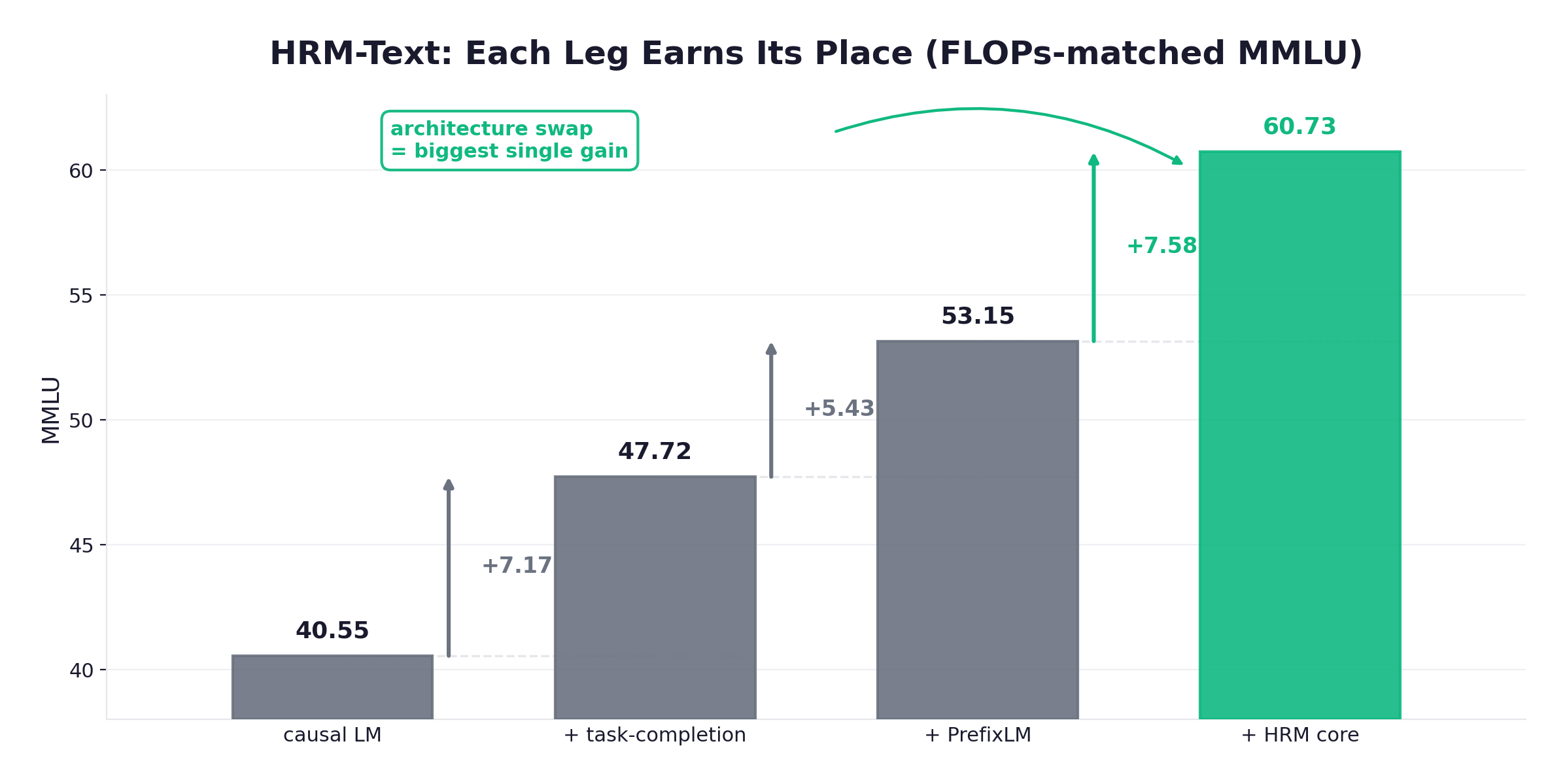
What it does not claim
Be honest about the ceiling. HRM-Text uses a fixed H2L3 schedule by design. ACT was explicitly removed, so depth is constant regardless of how hard the input is (the gap I will call Gap A in chapter 14). The inference-time auto-guidance trick is not test-time compute scaling: it only linearly combines logits from a fixed-depth loop at zero overhead, with small gains and a best w that varies per benchmark. The whole setup is offline, single-trajectory, deterministic: single-prompt conditional generation with no environment feedback, no online RL, no weight updates during interaction. And knowledge breadth stays bound by scale and data, the one axis depth cannot rescue.
HRM-Text internalizes the loop into language-model weights by deleting the tokens that carried it; chapter 11’s RLM is the opposite design, recursion pushed entirely outside.
11. RLM: The Counterpoint
The honest opposing bet: freeze the model, and let it write code that calls itself.
Chapters 7-10 put the loop in the weights. So now I want the cleanest possible counterargument, the bet that the loop should never enter the weights at all.
That bet is Recursive Language Models (RLM), from MIT CSAIL: Alex L. Zhang, Tim Kraska, and Omar Khattab (github.com/alexzhang13/rlm). RLM is my L2 representative, recursion in the harness, not in the network. It is the externalized counterpoint that makes the whole internalize/externalize choice concrete, and it shows me exactly what externalization is irreplaceably good at.
The mechanism: a prompt is an environment, not an input
The core move is a refusal. Instead of feeding a long prompt P into the network, RLM treats P as part of the environment the model interacts with. It boots a persistent Python REPL, stores the prompt as a variable named context, and lets the root model see only constant-size metadata: the length, a short prefix, and how to access it. The full string never enters the root’s context window. The window limit is sidestepped, not stretched.
From there the root writes code. The control loop is small: seed history with metadata, then while not done, the root emits a code snippet, the REPL executes it, and only a truncated prefix of stdout gets appended back to history. The loop ends when the root sets a Final variable. This is the Algorithm 1 skeleton:
Plain-text sketch of the RLM control loop. The prompt stays a REPL variable and the root only ever sees metadata.
       Input: prompt P   Output: response Y
state ← InitREPL(prompt=P)            # P stored as REPL variable `context`
state ← AddFunction(state, sub_RLM_M) # inject llm_query / rlm_query
hist  ← [ Metadata(state) ]           # root sees only constant-size metadata
while True:
    code            ← LLM_M(hist)             # root writes a code snippet
    (state, stdout) ← REPL(state, code)       # execute, update REPL state
    hist ← hist ∥ code ∥ Metadata(stdout)     # append only truncated stdout metadata
    if state[Final] is set: return state[Final]
The defining feature is symbolic recursion: code inside the REPL can invoke the model on programmatically constructed slices of P, inside a real for loop, rather than the model verbally delegating a fixed number of subtasks. Because it is real code, RLM can launch or even sub-calls. The slogan the authors use: if you can write a for-loop, you can do semantic aggregation, moving the workload out of one forward pass and into program time complexity. A single root turn is bounded, roughly total budget over per-turn truncation , but the real compute comes from sub-call count, which the for-loop scales with the prompt.
Depth is the externalized analogue of latent iteration count. It is a discrete dial 0/1/2/3, default depth=1. depth=0 has no sub-calls (REPL only, but can still offload the prompt); depth=1 calls a sub-LLM via llm_query, which ingests roughly 500K characters per call; depth>1 calls a sub-RLM via rlm_query, spawning a full child loop with its own REPL and falling back to llm_query at the cap. Recursion goes 0 to 3, and the “steps” are program loop iterations, not in-network ones.
Where it sits on the spectrum
This is the loop in code. Each adaptation is a full re-run, a fresh-context sub-call that shares no hidden state with its siblings. State persists as Python variables, not as vectors inside the network. That is the polar opposite of HRM/TRM, where each adaptation is a latent iteration.
And the externalized loop beats context-rot: the Context Rot (Hong et al., 2025) observation that quality degrades as the prompt grows even while it still fits the window. Programmatic recursion does not rot the way one forward pass does. The headline numbers, all median cross-benchmark margins for the GPT-5 variant:
| Comparison | RLM(GPT-5) median margin |
|---|---|
| vs context compaction | +26% |
| vs CodeAct with sub-calls | +130% |
| vs Claude Code | +13% |
On OOLONG-Pairs, a quadratic task, GPT-5 base scores 0.1 F1; RLM(GPT-5) hits 58.0 at depth=1 and 76.0 at depth=3. On BrowseComp-Plus (1K docs), GPT-5 base is 0.0 and RLM(GPT-5) depth=1 is 91.3, handling 6M-11M token inputs against a 272K window at an average of $0.99 per run.
Why externalization is genuinely strong
Here is the steelman chapter 12 has to weigh. Externalization buys three things a fixed-weight recursor cannot match. Extreme expressivity: 6M-11M tokens of input, output returned via a variable so length is unbounded too. Auditability: every step is code and stdout you can read, not a hidden vector you have to probe. Zero-shot pluggability: RLM wraps any base model, RLM(GPT-5) or RLM(Qwen3-Coder), with no retraining, no architecture surgery.
A conceptual orchestration sketch: recursion lives in the harness, every sub-call is a fresh-context forward pass, state lives in REPL variables.
       context = LONG_PROMPT            # >> any context window; never fed whole to root

def llm_query(text):             # depth=1: one fresh forward pass (~500K chars)
    return base_model(text)

def rlm_query(text, depth):      # depth>1: spawn a child RLM loop with its own REPL
    return run_rlm(text, depth - 1) if depth > 1 else llm_query(text)

# Omega(|P|^2) pairwise aggregation expressed as a for-loop over slices:
chunks = [context[i:i+K] for i in range(0, len(context), K)]
results = [rlm_query(a + "\n" + b, depth=2) for a in chunks for b in chunks]
Final = reduce(results)          # answer returned from a variable, unbounded length
I should be precise about what RLM does not claim. It is not an architecture paper: no gradient approximation, no fixed-point machinery, no differentiable halting. The “math” is a complexity argument plus standard rejection fine-tuning and RLVR, and halting is the root explicitly setting a variable. Recursion is not always good: on information-sparse CodeQA with Qwen3-Coder, depth=0 (66.0) beats every sub-call variant, and bad decomposition can backfire hard, with LongCoT-mini MATH degrading 26.0 to 5.6 without good hints. The REPL offload is the necessary condition for breaking the window; recursion is an extra knob that pays off mainly on information-dense, super-linear tasks.
There is even a convergence path: RLM-Qwen3-8B, rejection fine-tuned on 1072 trajectories, improves a median +28.3% across four tasks and runs more than 3x faster than the teacher. This is partial internalization, where the root gets better at orchestrating but the loop still runs at inference time.
Two clean opposites are now on the table: the loop in the weights, and the loop in the code. This sets up chapter 12, the head-to-head, where ARC-AGI-3’s scoring forces the question of where the adaptive loop should actually live.
12. Internalize vs Externalize
Run the slow self-rewriting Gödel loop outside in the harness and the fast “think a few more rounds” loop inside the weights, then let the benchmark’s scoring rule decide which one you are paying for.
Chapter 11 made the externalized case as strongly as it can be made. Now I want to take the opposite bet seriously and argue, against my own previous post, where the adaptive loop actually wants to live.
There are two routes for the “adapt to a novel environment” loop, and they sit at opposite ends of the L1/L2/L3 spectrum.
Externalize (L2). Adaptation lives in a self-rewriting harness. The Darwin Gödel Machine keeps an archive of agent variants, lets the LLM propose edits to its own scaffold code (tools, prompts, orchestration) and uses actual benchmark scores as fitness to keep or discard, with the model parameters frozen. The whole of my previous essay, From Singleton to System, was the systematic case for this route: internalize the kernel, externalize everything else. It showed a frozen base lifting SWE-bench Verified from 20.0 to 50.0 purely by evolving the harness.
Internalize (L3). Adaptation lives in latent depth recursion inside the weights: HRM, TRM, GRAM, HRM-Text. The loop carrier is internal latent recursion; the state is a hidden vector that is never emitted. HRM hits 40.3% on ARC-AGI-1 with 27M parameters, ~1000 samples, no pretraining and no CoT; TRM does it with 7M.
This post is the dual of the previous one. Last time I externalized adaptation into a self-evolving harness. This time I go inward.
The asymmetry: slow loop vs fast loop
The two routes have fundamentally different timing. Externalized adaptation is a slow loop: every rewrite re-runs and re-evaluates the whole agent. Internalized adaptation is a fast loop: the extra “thinking” happens within the same interaction tick, by deepening compute inside one forward pass.
| Externalize (L2, DGM/RLM) | Internalize (L3, HRM/TRM/GRAM) | |
|---|---|---|
| Adaptation carrier | outer scaffold code / orchestration | latent recursion over weight-tied block |
| Timing | slow: analyze → rewrite → re-run | fast: within one interaction tick |
| What changes | tools, prompts, code (model frozen) | hidden state (and, ideally, fast weights) |
| Expressivity | very high (10M+ tokens, arbitrary code) | bounded by recursion depth/width |
| Data efficiency | low (needs many eval rollouts) | extreme (~1000 samples, no pretraining) |
| Interpretability | high: auditable, every edit logged | low: latent never surfaces |
| Failure mode | reset/retry burns a full re-run | deeper but rigid if depth is fixed |
| Unit cost | ≈ one full re-run per adaptation | ≈ a few extra latent recursion steps |
Why ARC-AGI-3 tilts the table
ARC-AGI-3 is turn-based and interactive: the agent must discover rules and goals through multi-step interaction with a fresh environment and continually adjust its world model. Critically, it is scored on interaction efficiency. Every step is scored, and reset/retry costs scored steps, not wall-clock time.
That scoring rule changes the economics. “Slow” is suddenly fine, because nobody is timing your wall clock. The real cost is that each trial spends a scored step. And that is exactly where externalization bleeds: every strategy change in a DGM-style harness is a reset+retry, and each reset burns scored steps even if it is fast in seconds. The internalized loop, by contrast, deepens computation and adjusts the world model inside one interaction, consuming no extra scored step. HRM already shows the cheap half of this: trained with a recursion budget , you can raise it to 16 at inference and still gain accuracy. More depth, no retraining, no extra emitted tokens.
The bet, then: the adaptive loop wants to live in the weights, a Gödel-machine self-improvement loop moved out of code and into the weights.
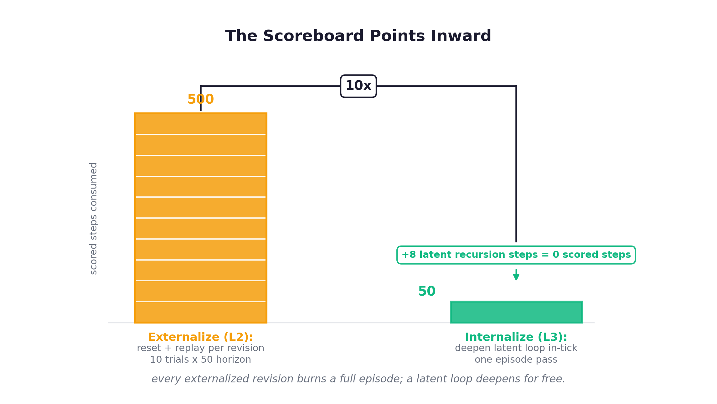
A tiny cost model makes the step-budget argument concrete. This is illustrative pseudo-code contrasting scored-step consumption of the two routes on a turn-based task.
       def scored_steps_externalize(trials, horizon):
    # each strategy revision = reset + replay the whole episode
    total = 0
    for _ in range(trials):           # one scaffold rewrite per trial
        total += horizon              # reset and re-run burns the full episode
    return total                      # ~ trials * horizon scored steps

def scored_steps_internalize(horizon, depth_train=8, depth_infer=16):
    # adaptation = deepen the latent loop inside the SAME interaction
    extra_depth = depth_infer - depth_train   # extra recursion, NOT extra steps
    _ = extra_depth                           # costs latent compute, 0 scored steps
    return horizon                            # one pass over the episode

print(scored_steps_externalize(trials=10, horizon=50))  # 500 scored steps
print(scored_steps_internalize(horizon=50))             #  50 scored steps
So under a step budget the internalized loop is asymptotically cheaper.
One honest qualification on that arithmetic, because it is easy to oversell. The gap is real only when the adaptation you need is more thinking about the observation you already hold. It is not a fair comparison when the environment hands you genuinely new information that overturns the plan. A deeper latent pass re-thinks what you have already seen; it does not, by itself, fold in what the environment returned a turn later. That cross-turn revision still needs an explicit history or a weight update, which is Gap B below, and it is exactly where the harness’s auditable, precisely replayable state stays the stronger tool. So read the scored-step win narrowly: L3 is cheaper for per-step reasoning depth, not a free substitute for updating a world model across turns.
Three honest counterpoints
There are three things the internalization papers do not claim, and I will not soften them.
One: current internalizers are offline, fixed-depth, and have no environment feedback. HRM, GRAM and HRM-Text are tested with frozen weights on offline, task-specific data. Their “adaptation” is single-forward latent refinement, multi-step thinking inside one pass, not a closed loop that updates a world model across interaction turns. To touch ARC-AGI-3 you would have to wire the latent loop to environment signals (reward, observation) via test-time training or fast weights. That wiring does not exist yet in these works.
Two: fixed depth is not fluid. HRM-Text does not even use ACT. Without an adaptive halting mechanism, more recursion is just deeper rigidity: every instance pays the same depth regardless of difficulty, which is the original fixed-depth pathology in a new costume. “Think harder only when it’s hard” has to be added (ACT on the depth axis, generative width via GRAM) or you have not built fluid intelligence, just a taller fixed ladder.
Three: externalization’s expressivity is a real, irreplaceable advantage. RLM proves it: 10M+ token contexts, symbolic recursion depth 0→3, fully auditable, zero-shot pluggable. A latent loop bounded by its recursion budget cannot match that ceiling. And HRM scores only 5.0% on ARC-AGI-2, so the internalized frontier is still narrow. The expressivity gap is not a rounding error.
Verdict: hybrid
So the pragmatic answer is not internalize-everything. It is hybrid: an internalized fast-adaptation kernel plus a thin external shell for tools, memory, and very-long context. Put the Gödel-machine slow loop outside in the harness, where its expressivity and auditability earn their keep; put the “think a few more rounds” fast loop inside the weights, where it can deepen within one scored interaction. The benchmark’s scoring rule tells you which loop you are being charged for, and on a step-scored, turn-based world, you want the cheap loop on the inside.
And the boundary may be subtler than weights against everything else. The kernel itself need not be a pure fixed point baked into parameters. It might be a half-internalized thing that still writes the occasional explicit pointer to its own context, a reflex that has learned when to externalize a note to itself rather than hold everything in latent state. Even the inside can keep a little outside, which is exactly the design I would bet on once Gap C below makes the cost of pure internalization plain.
But a kernel that adapts fast is only worth having if there is something rich for it to adapt, which raises the question of substrate: what the internal loop should actually run over.
13. The World Model Underneath
The previous post named the kernel worth keeping inside the weights, a world model and the loop that runs over it. Here the loop finally meets the model it runs on.
Chapter 12 argued the fast loop, the search-and-revise inner cycle, belongs inside the weights rather than bolted on as an external harness. But a loop iterates over something, and that something is a world model. This is where the two threads of the previous post converge.
The kernel was always two things
In From Singleton to System I ended on an open question: internalize the kernel, externalize the rest. But a kernel of what? My answer there was rough but I’ll commit to it now: the kernel is a world model plus the control loop that runs over it. Chapters 7 through 12 of this post supplied the loop: recurrent depth, latent iteration, learned halting. This chapter supplies the substrate the loop iterates against.
That a sequence model trained on nothing but next-token prediction grows a usable internal world model is not speculation. Othello-GPT is trained only to predict the next legal move on an 8x8 board, never told the board is 8x8 and never given piece colors, yet a linear probe recovers the board state and, the load-bearing part, a causal intervention along the probe direction actually changes the model’s subsequent legal moves. The representation is used, not merely correlated. Theory pushes in the same direction: Richens and Everitt prove that any agent robust to a distribution of tasks must have learned a causal world model, though crucially they do not prove that model has to be explicitly graph-structured. An implicit encoding in the weights satisfies the theorem too. So the world model is real and it can be implicit. The open question is whether you can read it out at the level you need.
What fluid intelligence actually demands
ARC-AGI-3 makes the demand sharp. It is a hidden-rule POMDP: the true transition and the goal are invisible, and the agent must identify them online. Human players clear it at 100%; frontier AI sits at an aggregate 0.51%. To move that number an agent has to do four things: build a world model from sparse observation, revise it the instant an observation contradicts it, discover the goal and a plan, and, between all of these, switch abstraction altitude. That last one is the bottleneck. On ARC the abstraction ladder runs pixel → object → relation → rule, and rules almost always live at the object/relation rung (“red block pushes blue block”). Stop at the pixel rung and the hypothesis space explodes into noise; abstract too aggressively and you throw away the recomposable structure. Choose the wrong altitude and the rule is invisible.
The mechanistic warning sign comes from the same Othello work. Li’s 2023 probe could only decode the board non-linearly under a black/white labeling. Nanda re-parameterized the identical activations as mine/theirs, where perspective flips each move, and the board became linearly readable and linearly intervenable. Same network, same activations, only the coordinate system changed, and the world model went from invisible to legible. Whether an emergent world model can be read out and causally used depends strongly on the altitude you query it at. ARC-AGI-3’s abstraction bottleneck is the exact same problem, just with the agent forced to find the right coordinate frame itself.
The central claim: altitude is depth
Here is the bet of this post, stated as plainly as I can.
A fixed-depth transformer reasons at a roughly fixed abstraction altitude. To climb higher it has to spend tokens. Chain-of-thought is the only altitude elevator it owns, and an expensive, brittle one. The HRM paper says it without flattery: CoT is a crutch, not a solution; one misordered step derails the whole chain. A looped or recurrent-depth model has a second elevator. It can iterate shared weights in latent space, refining the same hidden state, and each pass can lift the representation to a higher rung without emitting a single token.
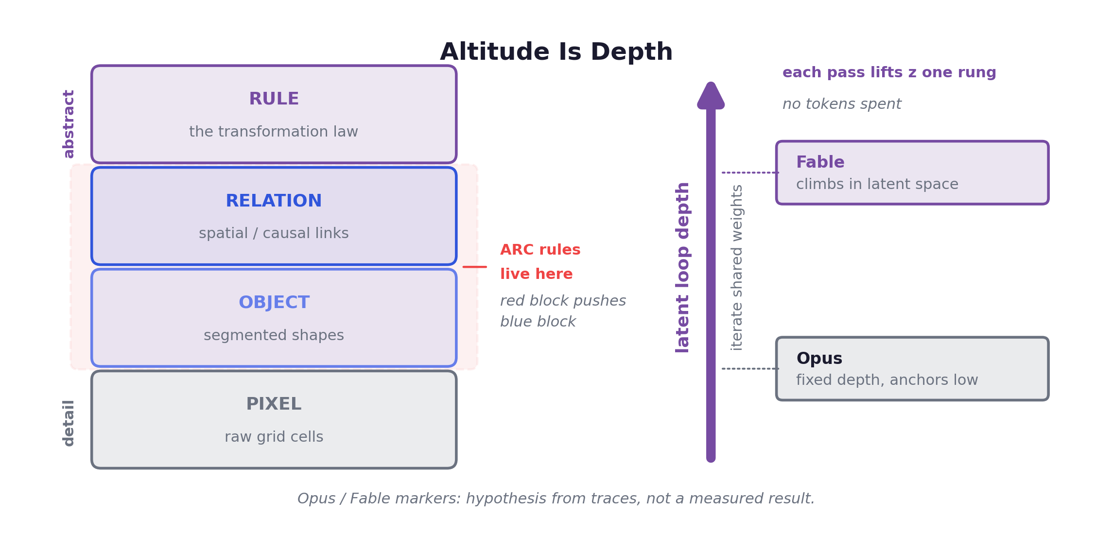
The strongest evidence we have that latent depth literally is altitude comes from HRM’s own internals (chapter 7). After training, the slow module’s representation spreads across far more dimensions than the fast module’s, the ~2.98x participation-ratio split from chapter 7, while an untrained network shows no split at all. So the high-dimensional abstract level is not wired in; it emerges, in the slow recurrent module, from training. The participation ratio is
over the eigenvalues of the hidden-state covariance, a soft count of how many dimensions the representation genuinely occupies. A high PR means the slow module spreads its state across many directions, the signature of an abstract code; a low PR means the fast module is committed to a narrow, detail-bound subspace. The slow recurrent loop is where altitude is gained. That is the mechanism behind the claim: climbing the abstraction ladder is iterating the recurrent core, and the rung you reach is set by how deep you let it loop.
I want to be careful. The HRM authors call the brain correspondence correlational, not causal, and the world-model framing for recurrent depth is mine, not theirs. The literature treats internal iteration as decision-time planning over an implicit model and never discusses recurrent-depth weights. The cross-link is conceptual. But the conceptual link is exactly the thing worth chasing.
The trace observation: a hypothesis, not a result
Now the anecdote, clearly flagged as my own hypothesis. Collecting Fable 5 traces on arc-witness-envs, a warm-up environment I built for exactly this kind of rule-discovery probing, the trajectories look markedly higher quality than Opus’s. The difference is not raw accuracy; it is altitude. The rules Fable proposes sit at the right level, governing rules about objects and relations, the rung where ARC rules actually live. Opus is short-sighted: it settles for low-level surface rules, fitting the pixels in front of it rather than the rule generating them.
The gap is concrete enough to read straight off the two models’ own words. Take two path puzzles from the same environment. On a stars puzzle, Opus writes down “reach the target cell,” reading the whole board as a maze, while Fable writes “pair same-color stars,” the rule that actually decides the win. On a color-separation puzzle, Opus reaches for button-mashing some win trigger while Fable states the partition rule outright. Same game, same frames, two very different rules written into each model’s reflection.
The line along the bottom of that comparison is the whole post in one sentence: low-level rules do not transfer to new layouts, so I distill the mechanism-true traces into the policy and shelve the surface ones. Internalize the governing rule, not the pixels.
My mechanistic reading: short-sighted is shallow, right-altitude is deep. Opus reasons at a fixed altitude and, lacking enough latent climb, anchors at the pixel/object boundary where the binding problem (Greff 2020) traps grid-reading models. Fable behaves like a model that can climb in latent space before it commits a hypothesis, a deep latent search reaching the relation/rule rung. This is a hypothesis with the shape of an explanation, not a measured result; a single trajectory’s “quality” is a judgment call, and I have no ARC-AGI-3 number for Fable yet. But it is the cleanest story I have for why altitude and depth keep coinciding.
A latent rollout probe
If the loop runs over a world model, you should be able to make it imagine. The schematic below iterates the recurrent core forward under a candidate action: a latent rollout, the world-model probe that connects recurrent depth to planning.
A candidate action is imagined by rolling the shared recurrent core forward in latent space and reading the predicted next state off a probe.
       # Latent imagination: roll the recurrent core under a candidate action,
# predicting the next latent state without touching the real environment.
def latent_rollout(core, head, z, action_emb, depth):
    z = z + action_emb            # inject the hypothesized action
    for _ in range(depth):        # climb: iterate shared weights in latent space
        z = core(z)               # each pass can lift z to a higher abstraction rung
    return z, head(z)             # predicted next latent state + decoded observation

def imagine(core, head, z0, candidate_actions, depth, emb):
    # score each candidate by rolling it out inside the model's own world model
    return {a: latent_rollout(core, head, z0, emb(a), depth) for a in candidate_actions}
# Deeper rollout = higher altitude of the imagined consequence. No tokens spent.
This is decision-time planning moved inside the weights: pick an action, imagine its consequence by looping the core, read off the predicted latent. The catch, the one chapter 14 has to confront, is that rolling out against an implicit world model with no falsifiable interface lets the model hallucinate its own rollout, and error compounds with depth, exactly as long CoT does over an implicit map. Chapter 14 turns to what is still missing to make altitude-by-depth real on ARC-AGI-3, and states the bet plainly.
14. What’s Missing, and the Bet
The four papers are an existence proof, not a finished engine, and the two pieces still missing are exactly the two that turn a loop from rigid into fluid.
If chapter 13 was right that abstraction altitude is latent depth, then the natural next move is to ask whether the loops we have actually let a model climb on demand. The honest answer is: not yet, not all the way.
Let me state plainly what the internalizers do prove. HRM trains from random init on roughly 1000 input-output examples per task, with no pretraining and no CoT supervision, at about 27M parameters, and lands 40.3% on ARC-AGI-1, ahead of models orders of magnitude larger (the full table is in chapter 7) while a same-setup direct-prediction Transformer scores a flat 0%. TRM does it at 7M params by simplifying HRM and beating it. GRAM adds a width axis, the N=20 trajectories beating a 320-step deterministic baseline from chapter 1. The shared lesson is not “a new SOTA”. It is that you can compile a search / multi-hypothesis / error-correction loop directly into the weights, that this is wildly data-efficient, and that it gives you exactly the inductive bias fluid intelligence needs: build a world model (ability #1) and revise it (ability #2). HRM trained at M_max=8 and raised to 16 at inference still gains accuracy with no retraining. The loop genuinely lives in the weights, as latent-state iteration, not in tokens and not in a harness.
Now what they do NOT prove. Every one of these systems is offline, fixed-depth per task, and has no environment loop. HRM inputs one puzzle and outputs one grid; there is no cross-step world-model update and no reward-driven online adaptation. Its Q-learning decides only how many segments to halt at, not how to interact with anything. The paper does not even mention ARC-AGI-3. The “adaptation” on offer is multi-step latent refinement inside a single forward pass. That is real, and it is not the same thing as adjusting a world model across turns of a fresh interactive environment. Two gaps stand between here and ARC-AGI-3.
Gap A: input-adaptive compute (ACT done right)
The whole premise is that effective computational depth should scale with instance difficulty: easy puzzle, few serial steps; hard puzzle, many. A fixed-depth Transformer nails that quantity to the architecture regardless of difficulty, which is the root pathology. The fix is adaptive halting, and the field is uneven on it. HRM has ACT (a Q-head over halt/continue). HRM-Text dropped it, which makes it deeper rigidity rather than fluid. GRAM’s “width” is parallel repeats, not adaptive depth. Mixture-of-Recursions points the cleaner way: a router decides per token how many recursion passes to spend, reframing ACT as routing over reuse counts of the same shared layers. Gap A is making the loop think harder only when it is hard, reliably, per instance, not on average.
Gap B: update the world model DURING interaction
This is the deeper gap. Today’s internalized adaptation lives entirely in activations and latent state. Nothing flows back into the weights, and nothing is wired to environment reward or observation. ARC-AGI-3 is turn-based: discover rules and goals through multi-step interaction with a fresh environment, continually adjusting the world model, with every step scored. Reset and retry cost scored steps, not wall-clock time, which is the whole scored-step economics of chapter 12, the reason the loop wants to live inside. Closing Gap B means a real in-interaction update: test-time training, fast weights, or online RL, with the inner update conditioned on what the environment just returned.
Here is a sketch of what is NOT yet built, a schematic in-interaction adaptation loop, to make Gap B concrete:
A speculative loop: observe the env, take a few inner fast-weight steps wired to that observation, then act. None of the four papers implement this.
       # SKETCH — not implemented by HRM/TRM/GRAM/HRM-Text. Illustrative only.
def in_interaction_adapt(policy, env, inner_lr):
    obs = env.reset()
    fast_w = policy.clone_adaptable_weights()        # fast weights, separate from base
    done = False
    while not done:                                  # each turn costs a SCORED step
        # Gap A: depth varies with how surprised we are by this observation.
        for _ in range(policy.act_halt_budget(obs)):
            pred = policy.predict_next(obs, fast_w)   # latent world-model rollout
            surprise = policy.consistency_loss(pred, obs)
            grads = torch.autograd.grad(surprise, fast_w)  # Gap B: update DURING interaction
            fast_w = [w - inner_lr * g for w, g in zip(fast_w, grads)]
        action = policy.act(obs, fast_w)
        obs, reward, done = env.step(action)         # reward/obs feed the NEXT inner update
    return fast_w                                    # the model that walked out is not the one that walked in
Gap C: credit assignment through a latent loop
There is a third gap, and it is the one that nags at me most, because it is where the two halves of this post pull against each other. Chain-of-thought won not because people enjoy reading it, but because a discrete, legible token trace is the substrate that makes credit assignment tractable. You can attach a process or outcome reward, see which step went wrong, and push gradient right at it. That is exactly how the composition results in Part II were earned: SPIRAL, the f-composition work, and Atomic-to-Composite all install composition with RL into models that still emit tokens. Internalize the loop into latent depth and you delete that legible action space. The reward now has to thread through dozens of opaque recurrent steps with no per-step handle to grab.
This is not hypothetical. It is why every internalizer in this post is trained with dense supervision on strong-label puzzles rather than sparse RL through the loop. HRM-Text can strip its chain-of-thought only because a next-token target still supervises every position; replace that dense signal with a sparse, outcome-level reward and the trick gets much harder. So the uncomfortable truth is that the mechanism most able to grow the kernel, reinforcement learning, is the one that latent internalization makes hardest to apply. Closing Gap C means either learning to assign credit through latent depth, or keeping a thin discrete scratchpad precisely for the steps a reward has to reach. Either way it points at the same place as the other two gaps: a hybrid, not a pure loop in the weights.
Testable hypotheses
I would bet on these, and they are falsifiable:
| Hypothesis | What would confirm it |
|---|---|
| Depth = fluid, per scored step | Adding latent recursion steps lifts ARC-AGI-3 score per scored step more than adding CoT tokens does |
| ACT is the key switch | An ACT-equipped loop beats a fixed-depth one of equal mean compute; HRM-Text-style “no ACT” stays brittle |
| Multi-hypothesis resists misleading rules | GRAM-style width survives deliberately deceptive demos where single-trajectory models lock onto a wrong surface rule |
| In-weight online adaptation beats external rewrite under a step budget | Fast-weight in-interaction updates outscore L2 reset-and-retry when every step is scored |
| H-module dimensionality tracks rule altitude | The slow module’s participation ratio rises when the discovered rule is more abstract |
| Credit assignment survives internalization | RL through a latent loop matches token-CoT RL on a composition task, or a hybrid scratchpad closes the gap where pure latent RL stalls |
That last one connects straight back to chapter 13: the ~2.98x emergent split from chapter 7, the altitude-is-depth bet, and the Fable-vs-Opus altitude gap in my arc-witness-envs traces. HRM is what that climb looks like in miniature, and (I’ll keep flagging it) the trace reading is my hypothesis, not a measured result.
Where the two halves meet
Step back and the two threads of this post collapse into one claim. The reasoning-primitives half said the kernel is atomic operations plus the control logic that composes them, that composition is the bottleneck, and that the lever which makes new compositions appear is the environment: primitives show up in a policy only when a task demands them. The recurrent-depth half said the composing loop can live in latent depth, trained at constant memory and deepened on demand. Put them together and the research program writes itself: reinforcement learning under environmental demand is how the kernel grows the compositions; recurrent depth is where the composed loop can run cheaply, once per scored step instead of once per re-run. SPIRAL and the f-composition results already show RL installing composition into an ordinary transformer’s weights; what nobody has built is the version where the loop doing the composing is itself adaptive in depth and updatable online. The environment is the teacher, the latent loop is the thing being taught, and the open frontier is wiring the teacher to the loop while the game is still being played. That is Gap A, Gap B, and Gap C, restated as one sentence.
The bet
So here is the bet, restated as the dual of From Singleton to System: last time the move was to externalize adaptation into a self-evolving harness; this time the move is inward. A Gödel-machine-style self-improvement loop, taken out of code and put into the weights. The Darwin Gödel Machine froze the model and evolved the scaffold; the bet here freezes nothing and lets the kernel adapt itself. Community reconstructions like OpenMythos speculate that recent Claude models lean looped / recurrent-depth (explicitly unconfirmed, not from any leak), and if the bet is right, this is exactly where it should show up: on fluid-intelligence tasks. The number I am actually waiting on is Fable 5’s ARC-AGI-3 score. If it lands well above the near-zero frontier, the direction holds; if it doesn’t, the traces were telling me something narrower than I think.
The loop, then, is the load-bearing kernel, the one thing worth internalizing, while the notebook stays outside as the external brain for everything else, which is where the closing picks up.
Closing: The Kernel Is a Loop Over Primitives
Last post I said internalize the kernel and keep a notebook for the rest. I just spent fourteen chapters arguing what the kernel actually is: reasoning primitives, and the loop that composes them.
Here is the whole post in short. The kernel has a substance and a mechanism. The substance is a small set of reasoning primitives plus the control logic that chains them, and the hard, transferable part, the part imitation cannot install, is the composition, which RL grows only when an environment demands it. The mechanism is a loop, and everything that makes a model think harder is one move: run that loop a few more times before answering. The only real choice is where the loop runs: in the tokens, in the harness, or in the weights. Chain-of-thought puts it in the tokens and pays in fragility and serial latency. The Darwin Gödel Machine and RLM put it in the harness and pay in re-runs. A looped, recurrent-depth network puts it in the weights and pays in training pain and lost interpretability. For a turn-based, step-scored, rules-not-announced task (fluid intelligence, in its purest operational form) the arithmetic of the scoreboard points at the weights, the scored-step case from chapter 12.
The deepest thing I take from putting the two halves side by side is that they are the same object. The control logic that composes primitives is a loop; the loop you internalize is the thing that composes them. When HRM, trained on a thousand puzzles, spontaneously does depth-first search with backtracking in its latent state, it is running exactly the control primitives the composition literature said were the hard thing to internalize. Not as tokens, not as a scaffold, but as iterated weights. The environment grows the compositions; recurrent depth is where they can cheaply live.
The recursive-LLM line is the existence proof that this is buildable. HRM internalized search and backtracking into 27M parameters and broke puzzles that crystallized giants score zero on. TRM stripped it to 7M and a single tiny network and did better, which told us the load-bearing part was the recursive refinement, not the elaborate machinery. GRAM made the loop keep several hypotheses alive instead of marrying its first guess. HRM-Text ported the whole idea to language and then deleted the chain-of-thought from its own training data, just to prove the reasoning could live in latent depth instead of tokens. None of this needed a bigger base model. It needed a loop, in the right place.
And then the honesty, because the bet is a bet. These models are still offline, fixed-depth, and blind to the environment between forward passes. They prove you can internalize a reasoning loop; they do not yet prove you can internalize an adapting one, a loop that deepens itself only when the puzzle is hard, and that updates its world model from what the environment just did. Those two gaps, input-adaptive compute and in-interaction adaptation, are exactly the two that separate a deep network from a fluid one. Nobody has closed them. The externalized shell, meanwhile, keeps a real and possibly permanent advantage on everything that is long, auditable, or changes faster than you can retrain. The endgame I actually believe in is not the weights winning. It is a hybrid: a thin Gödel-machine shell on the outside running the slow self-rewriting loop, wrapped around a kernel that has internalized the fast one.
I will tell you what tipped me from “interesting papers” to “I think this is the axis.” I have been collecting traces of Fable 5 playing arc-witness-envs, the little gym I built around Chollet’s framing, and the trajectories are a different animal from Opus: the rules Fable finds sit at the right level of abstraction while Opus settles for surface patterns. That altitude is the whole game in fluid intelligence, and altitude is depth (chapter 13). HRM hands you the mechanistic rhyme for free, the slow module spontaneously climbing to a higher abstraction level in the recurrent loop. Community reconstructions like OpenMythos guess that recent Claude models lean looped or recurrent-depth; that is explicitly unconfirmed and not from any leak, and I am holding it loosely. But if the bet is right, recurrent depth should keep widening the gap on exactly the tasks where abstraction altitude is decisive.
So this is my answer to the question I left open last time. Internalize the kernel, externalize the rest, and the kernel worth internalizing is the reasoning primitives and, above all, the loop that composes them: the fast, adaptive, altitude-climbing search that a notebook cannot serve in time. Keep the notebook, the perfect, unbounded, cloneable external brain, for everything else. That is not a smaller version of the Singleton. It is the System with its one irreducible reflex finally moved inside.
I do not know whether the first model to crack an ARC-AGI-3 environment without a task-specific harness will get there by looping its weights or by some trick I haven’t read yet. I do not know how much of the slow loop ever deserves to come inside. Those are the open questions, and they are why this is the most fun the field has been since pretraining first scaled. If you are working on recurrent depth, adaptive computation, test-time training, or the gym that would actually test any of it, come find me. I am on X, and I would rather argue about this in the open than be right alone.
I am still genuinely waiting on Fable 5’s ARC-AGI-3 number. If the loop belongs in the weights, that is where we will see it first.
References
Recurrent depth, latent reasoning, and the internalizers
- Hierarchical Reasoning Model (HRM), Wang et al., Sapient Intelligence + Tsinghua, 2025. arXiv
- Less is More: Recursive Reasoning with Tiny Networks (TRM), Jolicoeur-Martineau, Samsung SAIL Montréal, 2025. arXiv
- Generative Recursive Reasoning Models (GRAM), Baek, Jo, Kim, Ren, Bengio, Ahn, 2026. arXiv
- HRM-Text: Efficient Pretraining Beyond Scaling, Wang et al., Sapient Intelligence + MIT, 2026. arXiv
- Scaling up Test-Time Compute with Latent Reasoning: A Recurrent-Depth Approach (Huginn), Geiping et al., 2025. arXiv
- Mixture-of-Recursions: Learning Dynamic Recursive Depths for Adaptive Token-Level Computation, Bae et al., 2025. arXiv
- Universal Transformers, Dehghani et al., University of Amsterdam / DeepMind / Google Brain, 2018.
- Looped Transformers are Better at Learning Learning Algorithms, Yang et al., 2023.
Equilibrium and adaptive computation
- Deep Equilibrium Models, Bai, Kolter, Koltun, NeurIPS 2019. arXiv
- Adaptive Computation Time for Recurrent Neural Networks, Graves, 2016. arXiv
- PonderNet: Learning to Ponder, Banino et al., DeepMind, 2021. arXiv
Reasoning primitives and composition
- Faith and Fate: Limits of Transformers on Compositionality, Dziri et al., NeurIPS 2023. arXiv
- Skill-Mix: A Flexible and Expandable Family of Evaluations for AI Models, Yu et al., ICLR 2024. arXiv
- From f(x) and g(x) to f(g(x)): LLMs Learn New Skills in RL by Composing Old Ones, Yuan et al., ICLR 2026. arXiv
- Atomic Skills are the Prerequisite: When RL Synthesizes Compositional Reasoning (a.k.a. From Atomic to Composite), Cheng et al., ICLR 2026 Workshop SPOT. arXiv
- SPIRAL: Self-Play on Zero-Sum Games Incentivizes Reasoning via Multi-Agent Multi-Turn RL, Liu et al., ICLR 2026. arXiv
- Cognitive Behaviors that Enable Self-Improving Reasoners, Gandhi et al., 2025.
- Chain-of-Thought Prompting Elicits Reasoning in Large Language Models, Wei et al., 2022.
Externalized recursion and self-improvement
- Recursive Language Models (RLM), Zhang, Kraska, Khattab, MIT CSAIL, 2026. arXiv - code
- Darwin Gödel Machine, Zhang, Hu, Lu, Lange, Clune, 2025. arXiv
World models, abstraction, and fluid intelligence
- On the Measure of Intelligence, Chollet, 2019. arXiv
- Emergent World Representations (Othello-GPT), Li et al., ICLR 2023. arXiv
- DeepSeek-R1: Incentivizing Reasoning Capability in LLMs via Reinforcement Learning, DeepSeek-AI, 2025. arXiv
- ARC-AGI-3: A New Challenge for Frontier Agentic Intelligence (technical report), ARC Prize Foundation, 2026. arXiv
This series
- From Singleton to System-level Architecture (previous post), 2026. blog
The community reconstruction referred to in-text as OpenMythos is cited only as explicitly unconfirmed speculation, not from any leak, and has no canonical reference.