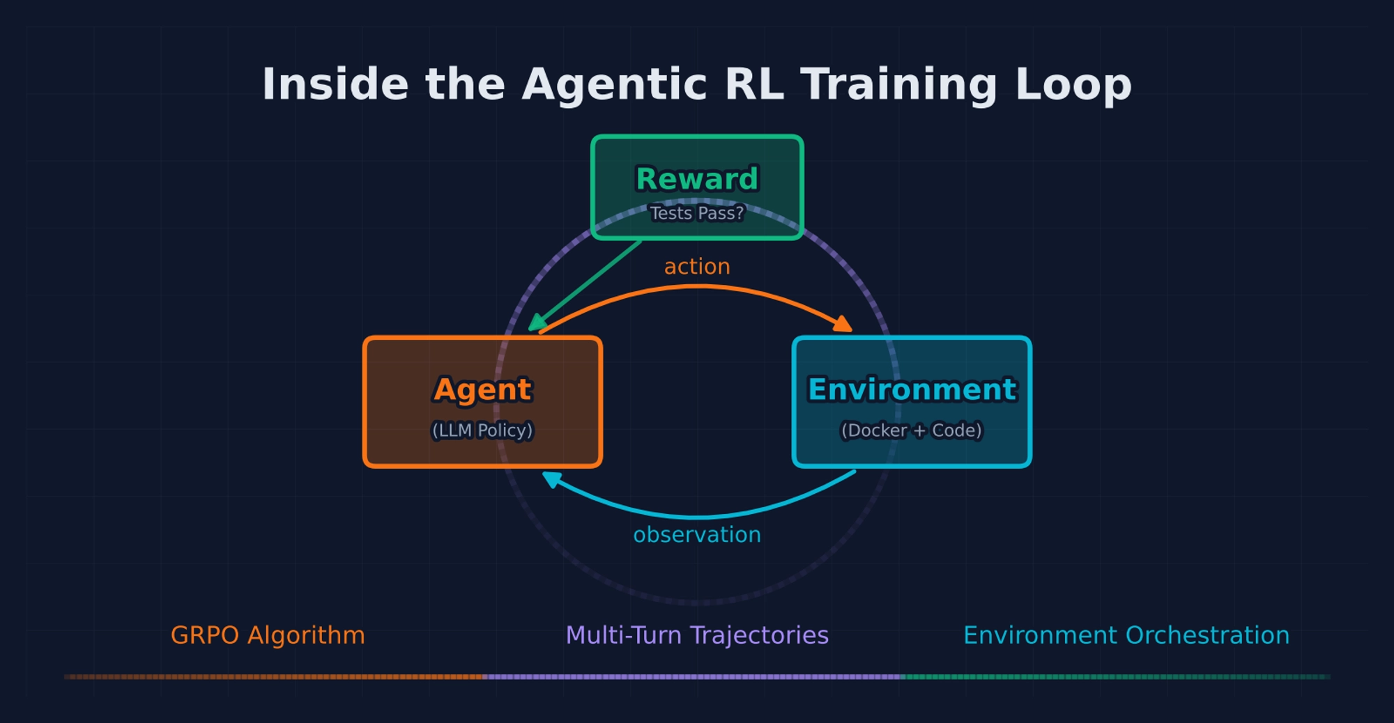
The algorithm is well-understood — GRPO with binary reward. The real complexity lives in everything else: how a multi-turn trajectory becomes a training sample, how loss masks determine which tokens receive gradients, how Docker containers are orchestrated at scale, and why training a single agent works for multi-agent deployment.
Over the past year, I’ve been digging into native agentic RL — the kind of RL that bakes agentic capabilities (tool use, multi-step planning, error recovery) directly into model weights, rather than relying on external scaffolding and prompt engineering. The recent release of GLM5 — one of the strongest open-source models for agentic tasks (77.8% on SWE-Bench Verified), trained with Zhipu AI’s Slime framework — is a good occasion to write up what I’ve learned. This post documents the full pipeline, step by step: from what happens inside a single rollout to how hundreds of rollouts are orchestrated in parallel, from how a multi-turn trajectory is flattened into a single training sample to how GRPO extracts learning signal from groups of trajectories.
The reference framework throughout is Slime (Zhipu AI / THUDM), with SWE-Bench as the training benchmark. The ideas are framework-agnostic — the same pipeline structure appears in DeepSWE, SWE-RL, Agent-R1, and every other native agentic RL system I’ve studied — but Slime is a natural starting point given the GLM5 results.
Update (Feb 24, 2026): This post has been updated with practical techniques from the GLM-5 technical report, which scales asynchronous agentic RL to production. Key additions include: token-level trajectory preservation (TITO) for async correctness, double-sided importance sampling for off-policy correction, and version-based staleness filtering for noisy sample handling.
1. What Is Native Agentic RL
The Two Ways to Build an Agent
Before 2024, building an LLM-based coding agent meant taking a capable base model and wrapping it in external scaffolding — ReAct prompting, orchestration frameworks like LangChain or AutoGPT, hand-crafted system prompts that spell out tool-use conventions, and multi-step pipelines that manage the agent loop. The model itself didn’t know how to be an agent; the framework did the thinking about when to search, when to edit, when to test.
Native Agentic RL flips this. Instead of engineering agentic behavior from the outside, we train it directly into the model’s weights. Through RL with environment interaction, the model learns to use tools, plan multi-step solutions, recover from errors, and manage context — natively, without relying on external orchestration. The “native” qualifier is about where the agentic capability lives: in the weights, not in the scaffold.
| Approach | Agentic Capability Lives In | Pros | Cons |
|---|---|---|---|
| Scaffold-based | External code (prompts, orchestration) | Quick to prototype, model-agnostic | Brittle, limited by prompt engineering ceiling, can’t improve through experience |
| Native Agentic RL | Model weights (trained via RL) | Robust, learns from experience, discovers novel strategies | Expensive to train, requires environment infrastructure |
How It’s Trained: RLVR in Agentic Environments
The training methodology is RL with Verifiable Rewards (RLVR) — the same paradigm used for math reasoning, but applied to agent-environment interaction. The core idea: drop the model into a real task environment — a code repository with a bug, a terminal, a test suite — let it try to solve the task through multi-turn interaction, observe whether it succeeded, and use that outcome as the reward signal. No expert trajectories to imitate. No human labelers to score outputs. Just: did the tests pass?
| Training Paradigm | Training Signal | What the Model Learns |
|---|---|---|
| SFT | Expert demonstrations | “How the expert solves this” |
| RLHF | Human preference labels | “What humans prefer to see” |
| RLVR (math/reasoning) | Verifiable answer correctness | ”How to reason correctly” |
| Native Agentic RL | Task outcome in real environment | “How to use tools and complete tasks” |
Native Agentic RL combines two ideas: the RLVR training methodology (grounded reward from verifiable task outcomes) and the goal of producing natively agentic models (models that inherently know how to interact with environments). The reward on SWE-Bench is literally 1.0 if the agent’s patch passes all tests, 0.0 otherwise. No proxy, no learned reward model to be hacked. The signal is grounded in reality.
Why does this matter? Because SFT has a ceiling effect — the model can never exceed the quality of its demonstrations. Scaffold-based agents are limited by the quality of their prompts and orchestration. And RLHF’s reward model can be gamed. Native Agentic RL, in principle, has none of these limitations. The model discovers strategies through exploration, the reward is incorruptible (assuming your test suite is sound), and the resulting capabilities are baked into the weights — no scaffold required at inference time.
The Landscape
As of 2025, several frameworks have emerged for native agentic RL:
| Framework | Organization | Key Design Choice | Model Size | SWE-Bench Verified |
|---|---|---|---|---|
| DeepSWE | Agentica | Simplified pipeline + RepoGraph | 32B (Qwen3) | ~50.8% |
| SWE-RL | Meta FAIR | First RL-for-SWE paper, clean baseline | 70B (Llama3) | ~41% |
| Agent-R1 | USTC | R1-style reasoning for agents | 7B+ | — |
| VerlTool | Tiger AI Lab (on VERL) | Multi-tool RL integration | 7B+ | — |
A few things stand out. GRPO dominates — almost every framework uses it, because eliminating the value model simplifies infrastructure dramatically. Open-weight RL-trained agents have closed the gap with proprietary models — DeepSWE’s 32B model (~50.8%) matches Claude 3.5 Sonnet (~49%), a striking validation of the approach.
But the most impressive results come from production-scale systems training much larger models:
| System | Organization | Model | SWE-Bench Verified | Key Innovation |
|---|---|---|---|---|
| Slime | Zhipu AI | GLM-5 (744B / 40B active MoE) | 77.8% | Async training (integrates APRIL), 3-layer architecture |
| MiniMax Forge | MiniMax | M2.5 (230B / ~10B active MoE) | 80.2% | CISPO algorithm, tree-structured merging, process reward |
| VERL | ByteDance | General-purpose (tested at 671B) | — | 3D-HybridEngine, AgentLoopBase + VerlTool for agentic RL |
| Poolside Model Factory | Poolside | Proprietary | — | 10K H200 GPUs, Saucer (800K+ repos), end-to-end automation |
MiniMax Forge is particularly notable for its black-box agent integration — the framework intercepts the agent’s API calls without requiring any modification to the agent code itself — and its CISPO (Clipped Importance Sampling Policy Optimization) algorithm that clips importance weights while preserving gradients. Its tree-structured merging yields ~40x training speedup over naive sequential rollouts. Poolside’s system is the most complete end-to-end infrastructure publicly documented, with GPU-Direct NCCL transferring Llama 405B weights (810 GB) in ~2 seconds. For a deeper comparison of these infrastructure frameworks, see the companion post on RL infrastructure.
Worth noting: Zhipu AI (THUDM) maintains two complementary frameworks — Slime and AgentRL. Slime is the general-purpose RL training infrastructure (SGLang + Megatron) used to train the full GLM model family (GLM-4.5 through GLM-5), handling both reasoning and agentic capabilities. AgentRL is a higher-level framework specifically for multi-turn, multi-task agent training — it tackles challenges like heterogeneous environment orchestration, cross-policy sampling, and task advantage normalization, and was adopted to build AutoGLM. Where Slime answers “how to scale RL training efficiently across thousands of GPUs,” AgentRL answers “how to train agents that interact with diverse real-world environments (web, OS, APIs) across multi-turn episodes.” AgentRL’s benchmarks (AgentBench) are broader than SWE-bench, covering web browsing, OS operations, and other interactive tasks beyond coding.
What Makes Agentic RL Structurally Different from Math RLVR
If you’ve worked with RLVR for math or reasoning, agentic RL might look superficially similar — same algorithms, same training loop pattern. But the engineering challenges are qualitatively different:
| Dimension | Math / Reasoning RLVR | Agentic Coding RL |
|---|---|---|
| Environment | Stateless (verify the answer) | Stateful (Docker container with repo, deps, tests) |
| Episode length | Single generation, < 4K tokens | Multi-turn, 2K-128K tokens |
| Reward latency | Milliseconds | Minutes (run test suite) |
| Action space | Natural language | Tool calls (file_edit, terminal, search) |
| Parallelism | Trivial | Complex (container orchestration) |
| Credit assignment | Direct (output → reward) | Ambiguous (which of 15 turns caused success?) |
The stateful environment requirement is the defining challenge. For math RLVR, you can generate 1024 completions in a batched inference call and verify them in microseconds. For coding RL, each completion requires launching a Docker container, checking out a repository, running a multi-turn interaction loop, and executing a test suite. Wall-clock time per trajectory: 3-10 minutes, not 3-10 seconds.
2. The Framework: Slime’s Three-Layer Architecture
Most RL training frameworks were designed for single-turn RLVR: generate one completion, score it, update the policy. Agentic RL breaks this model — a single trajectory might take 5 minutes of wall-clock time across 10-25 interaction turns. If the training engine waits for all trajectories to complete, GPUs sit idle for minutes between gradient steps. (For a broader survey of how different organizations — Poolside, MiniMax, ByteDance, and others — approach RL training infrastructure, see my companion post on RL Infrastructure for Large-Scale Agentic Training.)
Slime’s answer is a three-layer architecture that separates concerns: Training, DataBuffer, and Rollout.
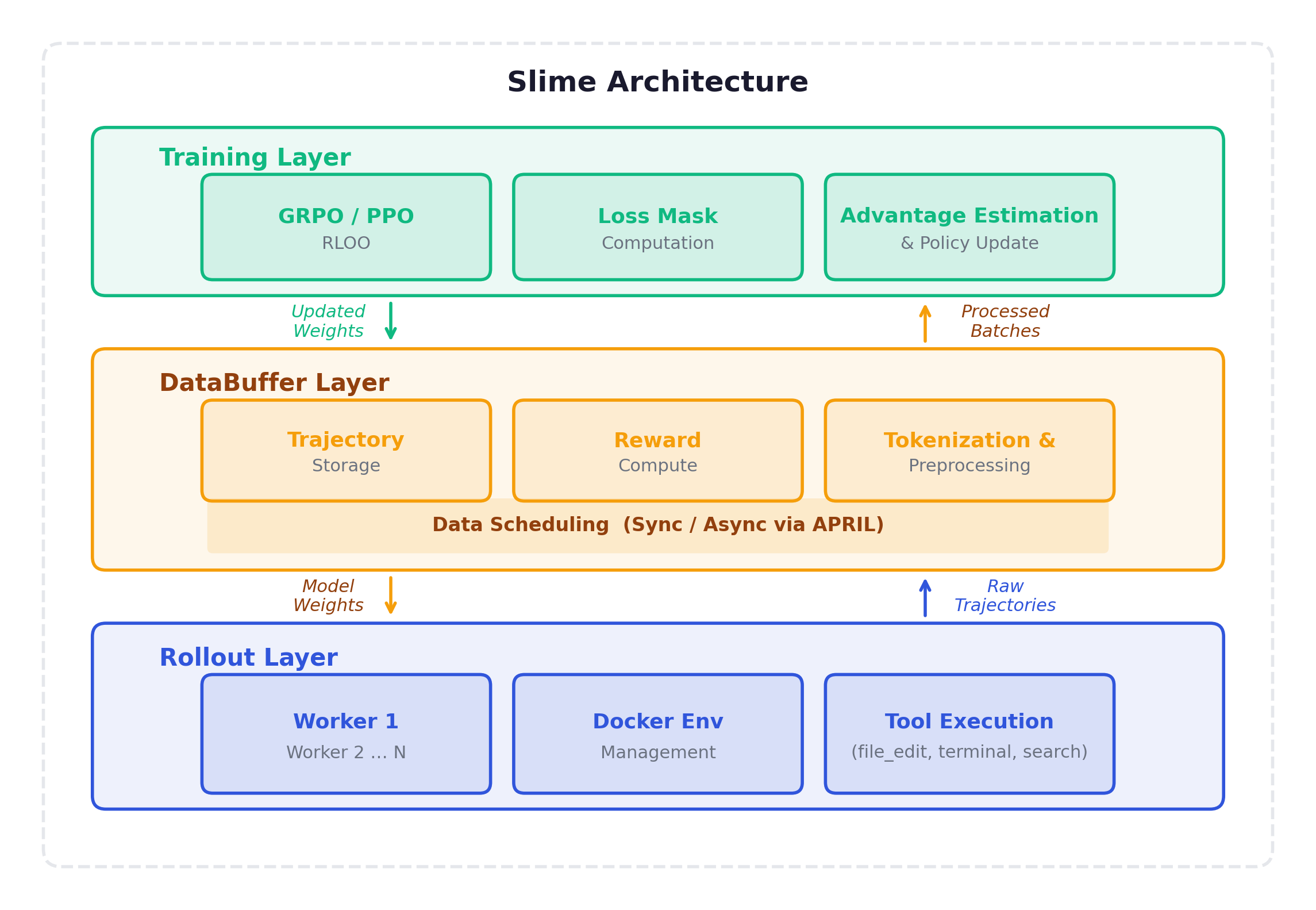
Training Layer manages the policy update — receive processed batches, compute GRPO loss, run backward pass, push updated weights. This is the simplest layer. It supports GRPO, PPO, RLOO, and GRPO++ (with length normalization to combat verbose trajectories).
DataBuffer Layer is the transformation pipeline: receive raw trajectories from workers, compute rewards, group by prompt for GRPO, tokenize multi-turn conversations into flat sequences, compute loss masks and advantages, filter degenerate trajectories, and assemble training batches. In async mode (APRIL), it continuously accumulates data and provides batches to Training as they become ready.
Rollout Layer is where the model interacts with the world. 32-128+ parallel workers, each managing a Docker container, running the agent loop (generate → execute → observe), collecting trajectories. This is the most complex layer and the one that consumes ~80% of wall-clock time.
Synchronous vs. Asynchronous (APRIL)
Slime integrates APRIL (Active Partial Rollouts in Reinforcement Learning), a system-level optimization from AMD/CMU/LMSYS/UCLA that addresses the long-tail generation bottleneck. The choice between sync and async is the most impactful architectural decision:
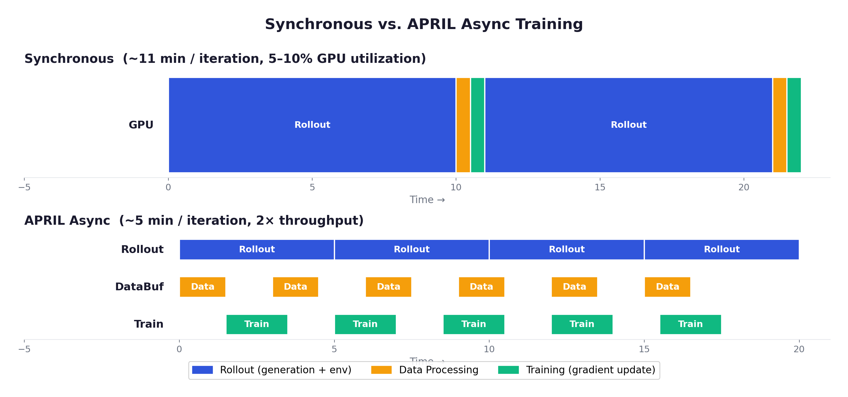
Synchronous: all workers complete → DataBuffer processes → Training updates → repeat. Clean and strictly on-policy, but GPU utilization is terrible — typically 5-10%, because training GPUs idle during the multi-minute rollout phase.
Asynchronous (APRIL): Rollout, DataBuffer, and Training all run concurrently. Workers continuously generate trajectories. Training continuously consumes batches. Result: ~2x throughput improvement.
The tradeoff is staleness — some trajectories in a batch were generated by an older policy version. APRIL mitigates this through importance sampling correction, staleness budgets (discard trajectories more than K steps old), and policy version tracking for precise ratio computation. In practice, the staleness is manageable because the KL penalty in GRPO keeps consecutive policy versions close.
GLM-5 takes a different approach to the async off-policy problem with direct double-sided importance sampling. The challenge: in async training, a single multi-turn trajectory may span multiple policy updates, so is not a single policy but a mix of versions. APRIL handles this through precise version tracking, which requires maintaining historical checkpoints or re-evaluating log-probs — expensive at scale. GLM-5 instead takes the simpler route: use the log-probabilities recorded during rollout directly as the behavior proxy, regardless of which policy version produced each token: . This is an approximation, but they bound the error with double-sided clipping — stricter than standard PPO’s asymmetric clip — where tokens falling outside this interval are entirely masked from gradient computation (set to zero, not clipped). This hard masking prevents extreme off-policy updates from destabilizing training, which is particularly important for long-horizon agentic trajectories where policy drift accumulates across many turns.
| How is obtained | Precision | Overhead | |
|---|---|---|---|
| Sync GRPO | Rollout log-probs = old policy (exact match) | Exact | None |
| APRIL (async) | Version tracking + precise IS correction | Exact | High (historical checkpoints) |
| GLM-5 (async) | Rollout log-probs as direct proxy (approximation) | Approximate | None; compensated by aggressive clipping |
Eight Extension Points
Slime provides 8 customizable function hooks covering the full pipeline — from generation format (custom_generation_fn) to reward computation (custom_reward_fn) to trajectory filtering (custom_filter_fn). This makes it possible to adapt the framework to new tasks without modifying core code:
       config = SlimeConfig(
    model=ModelConfig(model_name_or_path="Qwen/Qwen2.5-Coder-7B-Instruct"),
    training=TrainingConfig(algorithm="grpo", group_size=8, kl_coeff=0.01),
    rollout=RolloutConfig(num_workers=32, max_turns=50, timeout_seconds=600),
    reward=RewardConfig(reward_type="binary"),
    async_mode=True,  # Enable APRIL
)

trainer = SlimeTrainer(config)
trainer.register_reward_fn(custom_reward_fn)
trainer.register_env_fn(custom_env_fn)
trainer.register_filter_fn(custom_filter_fn)
trainer.train()
3. The End-to-End Training Pipeline
Let’s walk through a complete training iteration, from task sampling through policy update.
Phase 0: Data Preparation
Before training begins, we need a task pool and execution environments.
SWE-Bench provides GitHub issues with ground-truth test patches. After filtering out repositories that take >10 minutes to build, issues requiring external services, and tasks with flaky tests, a typical training pool contains 300-500 tasks.
The critical preparation step is pre-building Docker images — for each (repository, commit) pair, a Docker image with the full repo, all dependencies, and a configured test framework:
| Repository @ Commit | Docker Image | Size |
|---|---|---|
django/django@abc123 | swebench-django-abc123:latest | ~2-4 GB |
flask/flask@def456 | swebench-flask-def456:latest | ~1-2 GB |
Pre-building matters enormously: installing dependencies from scratch takes 5-30 minutes per repository. With pre-built images, container startup drops to 2-3 seconds. The initial image-building phase takes 2-4 hours with parallel builds, but only happens once.
Phase 1: Trajectory Generation (Rollout)
This is the bottleneck — ~80% of wall-clock time.
Sample a batch: With GRPO group_size G=8 and batch_size=64, we sample 8 unique tasks and generate 8 independent rollouts each.
Launch containers: Each of the 64 task-rollout pairs gets its own Docker container, checked out to the correct commit. With a pre-warmed pool: 2-3 seconds. Without: 30-60 seconds.
Run the agent loop (up to 50 turns per trajectory):
       client = OpenAI(base_url="http://sgl-router:8000/v1")  # Rollout engine

messages = [
    {"role": "system", "content": system_prompt},
    {"role": "user", "content": task.issue_text},
]

for turn in range(max_turns=50):
    response = client.chat.completions.create(
        model="policy", messages=messages, temperature=0.7
    )
    assistant_msg = response.choices[0].message.content
    action = parse_action(assistant_msg)
    observation = container.execute(action)

    messages.append({"role": "assistant", "content": assistant_msg})
    messages.append({"role": "tool", "content": observation})

    if action.type == "submit":
        break
A concrete example — fixing a Django bug where QuerySet.only() crashes with select_related():
| Turn | Agent (Thinking + Action) | Environment |
|---|---|---|
| 1 | <think>Need to find relevant code</think> <action>search: QuerySet.only</action> | query.py:1205 |
| 2 | <think>Read the implementation</think> <action>file_read: query.py:1200-1250</action> | def only(self, *fields): ... |
| 3 | <think>Found it — deferred_loading ignores related fields</think> <action>file_edit: compiler.py ...</action> | File edited successfully |
| 4 | <think>Verify the fix</think> <action>terminal: python -m pytest tests/</action> | 5 passed, 0 failed |
| 5 | <action>submit</action> | — |
Compute reward: Apply the ground-truth test patch to the container, run pytest, check results. Binary: 1.0 if all pass, 0.0 otherwise.
Package and submit: The trajectory (all turns + reward + metadata) is sent to the DataBuffer. With 32 workers in parallel, the full batch of 64 trajectories completes in roughly (64 / 32) × 5min ≈ 10 minutes.
Phase 2: Data Processing (DataBuffer)
Trajectories go through a transformation pipeline to become training-ready batches:
Group by prompt: GRPO needs all G=8 trajectories for the same task grouped together.
Tokenize: Each multi-turn trajectory is flattened into a single token sequence — system prompt, user prompt, and all (assistant, tool) turn pairs concatenated.
Compute loss masks: Binary mask over the token sequence — 1 for model-generated tokens, 0 for everything else. More on this in the next section.
Compute advantages: For each prompt group, GRPO normalizes rewards:
       rewards = [1.0, 0.0, 1.0, 0.0, 0.0, 1.0, 0.0, 0.0]  # G=8
mean_r, std_r = 0.375, 0.484
advantages = [(r - mean_r) / std_r for r in rewards]
# [+1.29, -0.77, +1.29, -0.77, -0.77, +1.29, -0.77, -0.77]
Successful trajectories get positive advantages (reinforced). Failed ones get negative advantages (suppressed).
Filter degenerates: Discard trajectories where all G rewards are identical (no signal), loops (approaching max turns with reward=0), or extreme lengths (>50K tokens).
Assemble batch: Package input_ids, loss_mask, advantages, old_log_probs, ref_log_probs into a training batch.
Phase 3: Policy Update (Training)
The actual gradient computation is straightforward:
       # Forward pass
logits = model(batch["input_ids"])
log_probs = compute_log_probs(logits, batch["input_ids"])

# GRPO loss
ratio = exp(log_probs - batch["old_log_probs"])
clipped_ratio = clip(ratio, 1 - 0.2, 1 + 0.2)
policy_loss = -min(ratio * advantages, clipped_ratio * advantages)

# KL penalty
kl_penalty = 0.01 * (log_probs - batch["ref_log_probs"])

# Apply mask and compute total loss
loss = ((policy_loss + kl_penalty) * loss_mask).sum() / loss_mask.sum()

loss.backward()
clip_grad_norm(model.parameters(), max_norm=1.0)
optimizer.step()
A single training step takes ~20-40 seconds. Compare this to the 10-minute rollout phase — the 20:1 ratio is why generation efficiency is the primary optimization target.
Timeline
A full training run (3 epochs, 500 tasks, G=8): ~188 iterations. Synchronous: ~34 hours. With APRIL: ~17 hours.
4. How Trajectories Become Training Data
This is the conceptually trickiest part of agentic RL. In single-turn RLVR, training data is simple: one prompt, one completion, one reward. The model produced one block of text, compute the policy gradient over it.
Agentic trajectories are messier. The model produces multiple blocks of text (one per turn), interleaved with environment responses it didn’t generate. The reward arrives only at the very end. How does the gradient actually flow?
One Trajectory = One Training Sample
A trajectory is not split into separate training samples. The entire multi-turn sequence is concatenated into a single token sequence:
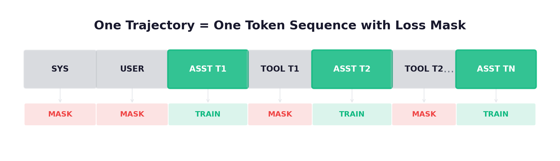
The model processes the full sequence in one forward pass. Loss masking determines which tokens receive gradients: only model-generated tokens (assistant turns) are trained on. Environment-generated tokens (system, user, tool) are in the sequence for context — the model sees them during the forward pass, which affects hidden states and therefore gradients on the assistant tokens — but they don’t directly contribute to the loss.
Loss Masking: The Core Mechanism
| Token Type | In Loss? | Reason |
|---|---|---|
| System prompt | No (mask) | Not model-generated — environment setup |
| User prompt | No (mask) | Not model-generated — task description |
| Assistant response (each turn) | Yes (train) | Model-generated — this is the policy |
| Tool observation (each turn) | No (mask) | Not model-generated — environment feedback |
All assistant turns are trained simultaneously. The masking is not progressive or per-turn by default. Turn 1’s assistant tokens, turn 5’s assistant tokens, and turn 15’s assistant tokens all receive the same advantage signal and are all updated in the same backward pass.
This is analogous to teacher forcing in seq2seq models: the model sees real observations (not its own predictions about what the environment would return) and learns what to do given those observations.
The Trajectory Data Structure
Before looking at examples, let’s see how a trajectory is represented in code. The data structures make the token-sequence-with-masking concept concrete:
       @dataclass
class Turn:
    """One turn in the agent interaction loop."""
    turn_index: int
    assistant_message: str      # Model output: thinking + action
    observation_message: str    # Environment response
    tokens_generated: int       # Tokens the model produced

@dataclass
class Trajectory:
    """A complete agent trajectory for one task."""
    task_id: str
    system_prompt: str
    user_prompt: str
    turns: List[Turn]
    reward: float
    metadata: Dict[str, Any]

    def to_token_sequence(self):
        """Convert to flat sequence with trainability labels."""
        segments = []

        # System prompt — NOT trainable
        segments.append({"role": "system", "content": self.system_prompt,
                         "trainable": False})
        # User prompt — NOT trainable
        segments.append({"role": "user", "content": self.user_prompt,
                         "trainable": False})

        # Each turn: assistant is trainable, tool is not
        for turn in self.turns:
            segments.append({"role": "assistant", "content": turn.assistant_message,
                             "trainable": True})    # <-- gradients flow here
            segments.append({"role": "tool", "content": turn.observation_message,
                             "trainable": False})   # <-- no gradients
        return segments
The to_token_sequence() method is the critical transformation: it converts a structured multi-turn conversation into a flat list of segments, each labeled as trainable or not. The tokenizer then converts this into input_ids and loss_mask tensors aligned token-for-token.
Token-in-Token-out (TITO) vs. Text-in-Text-out. In synchronous training, the above transformation is straightforward — the trainer tokenizes each trajectory from text. But in asynchronous setups, a subtle but consequential choice arises. The text-in-text-out approach treats the rollout engine as a black box that returns finalized text; the trainer then re-tokenizes it. This re-tokenization can introduce mismatches in token boundaries, whitespace normalization, truncation, or special-token placement — which in turn corrupts the alignment between actions and rewards/advantages. GLM-5 adopts the token-in-token-out (TITO) approach instead: the rollout engine emits the exact token IDs and metadata it produced, and the trainer consumes them directly. A TITO Gateway intercepts all generation requests, records each trajectory’s token IDs, and passes them through without any lossy text round-trip. This preserves exact action-level correspondence between what was sampled and what is optimized — critical when rollouts are streamed, truncated, or interleaved across many async actors.
A Worked Example
3-turn trajectory for fixing an IndexError:
| Turn | Role | Content |
|---|---|---|
| 1 (Search) | Assistant | Think: Need to find the file. Action: search: IndexError utils.py |
| Tool | utils.py:42: items[len(items)] # IndexError | |
| 2 (Fix) | Assistant | Think: Off-by-one. Should be len-1. Action: file_edit: utils.py ... |
| Tool | File edited successfully. | |
| 3 (Verify) | Assistant | Think: Run tests to verify. Action: terminal: pytest tests/ |
| Tool | 5 passed, 0 failed | |
| Reward | 1.0 |
The loss mask:
| Position | [0..50] | [51..80] | [81..130] | [131..200] | [201..240] | [241..270] | [271..310] | [311..330] |
|---|---|---|---|---|---|---|---|---|
| Content | SYS | USER | ASST_T1 | TOOL_T1 | ASST_T2 | TOOL_T2 | ASST_T3 | TOOL_T3 |
| Mask | 000… | 000… | 111… | 000… | 111… | 000… | 111… | 000… |
With GRPO (G=4 for this task):
| Trajectory | Outcome | Reward | Advantage |
|---|---|---|---|
| Traj 1 (above) | Tests pass | 1.0 | +1.15 |
| Traj 2 | Edited wrong file | 0.0 | -0.58 |
| Traj 3 | Tests pass | 1.0 | +1.15 |
| Traj 4 | Timeout | 0.0 | -0.58 |
Training effect: the model increases the probability of search → fix → verify patterns (Traj 1 & 3) and decreases the probability of misidentification (Traj 2) and looping (Traj 4).
The Credit Assignment Problem
The fundamental challenge: in a 15-turn trajectory that succeeds, which turns caused the success? Was it the search in turn 3? The fix in turn 7? The debugging cycle in turns 10-13?
GRPO’s approach is deliberately coarse: assign the same advantage to every assistant turn. If the trajectory succeeded, every turn gets a positive advantage. If it failed, every turn gets a negative advantage.
This seems wasteful. But it works for two reasons:
-
Signal averages out across iterations. Good strategies (search first, then fix, then test) appear in successful trajectories more often than in failed ones, so they get reinforced — just less strongly than the key actions.
-
The alternative is expensive. Per-turn credit assignment requires either a trained critic model (PPO/GAE, needing ~84 GB extra memory for a 7B model) or Shapley value computation (exponentially expensive). GRPO’s uniform assignment trades precision for simplicity.
For the research frontier: iStar estimates per-turn contributions using hindsight analysis. Progressive masking (training on only the last turn initially, then expanding) provides a curriculum-based middle ground. But the standard full-assistant-mask approach is what ships in production.
Five Masking Strategies
While the standard approach (full assistant mask) dominates, it’s worth knowing what alternatives exist — they may become important as the field matures:
| Strategy | What’s Trained | Use Case |
|---|---|---|
| Full Assistant Mask | All assistant tokens across all turns | Default. Simple, stable. Used by Slime, SWE-RL, DeepSWE. |
| Action-Only Mask | Only <action>...</action> tokens, not <think> | Focuses gradient on decisions. Risk: model doesn’t learn to reason. |
| Progressive Mask | Epoch 1: last turn only. Epoch 2: last 3 turns. Epoch 3: all. | Curriculum learning for long trajectories (50+ turns). |
| Outcome-Weighted | All assistant tokens, but with continuous weights (0.1–2.0) based on reward | Similar to GRPO advantage, redundant in practice. |
| Turn-Selective | Only turns scoring above a quality threshold | Requires per-turn scoring (critic or heuristic). Finest granularity. |
In code, the standard full assistant mask is trivial:
       def full_assistant_mask(tokens):
    """1 for assistant tokens, 0 for everything else."""
    return [1 if t.role == "assistant" else 0 for t in tokens]
The action-only mask is more selective:
       def action_only_mask(tokens):
    """1 only for tokens inside <action> tags."""
    return [1 if t.role == "assistant" and t.is_action else 0 for t in tokens]
The progressive mask implements curriculum learning:
       def progressive_mask(tokens, current_epoch, total_epochs, max_turns):
    """Gradually unmask more turns as training progresses."""
    progress = current_epoch / max(total_epochs - 1, 1)
    turns_to_unmask = max(1, int(progress * max_turns) + 1)
    max_turn = max(t.turn_index for t in tokens if t.turn_index >= 0)
    threshold = max_turn - turns_to_unmask + 1

    return [1 if t.role == "assistant" and t.turn_index >= threshold else 0
            for t in tokens]
The All-Same Problem
When all G trajectories for a task get the same reward (all succeed or all fail), advantages are zero — no gradient signal. Solutions:
- DAPO’s dynamic sampling: filter out zero-variance prompt groups entirely
- Curriculum design: maintain a mix of task difficulties
- Larger G: with G=16, the probability of all-same outcomes drops significantly
5. Environment Orchestration — The Hidden Bottleneck
If you’ve worked with math RLVR, environment orchestration isn’t something you’ve had to think about. The “environment” is a function that checks if 2 + 3 = 5. Stateless, instant, trivially parallelizable.
Agentic coding RL is different. The environment is a full software development setup — a cloned repository, installed dependencies, a working test suite, tool endpoints. Every trajectory requires its own isolated environment, and each takes seconds to minutes to set up. At scale, environment management becomes the primary engineering challenge.
The Docker Architecture
Every task-rollout pair gets its own container. This is non-negotiable:
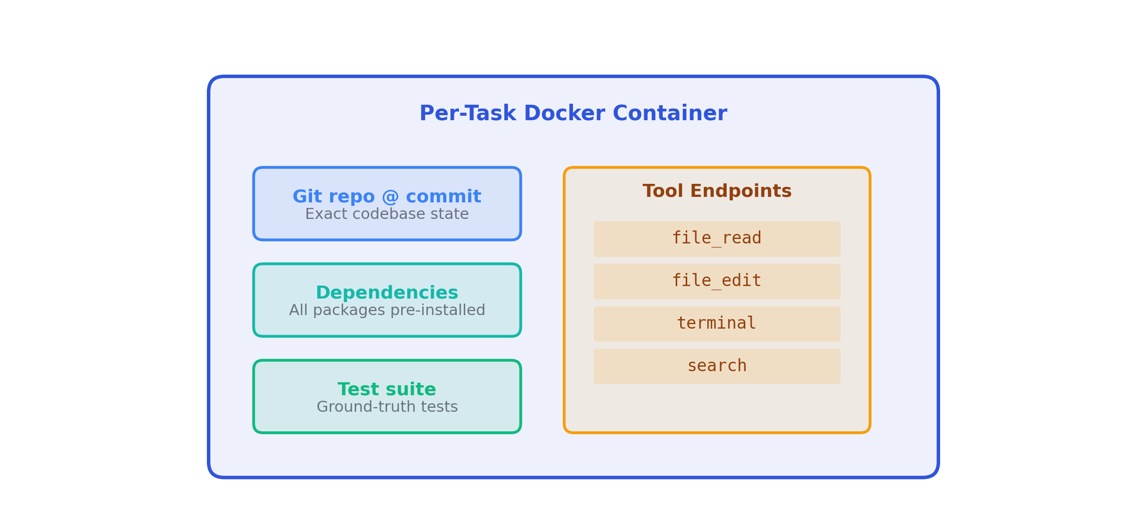
Isolation: Agent A’s file_edit must not affect Agent B’s environment. With G=8, eight containers run the same task concurrently, each accumulating different file edits.
Reproducibility: GRPO requires all G rollouts for a task to start from identical states.
Cleanup: After trajectory completion, the container is destroyed. No state leaks.
The Container Lifecycle
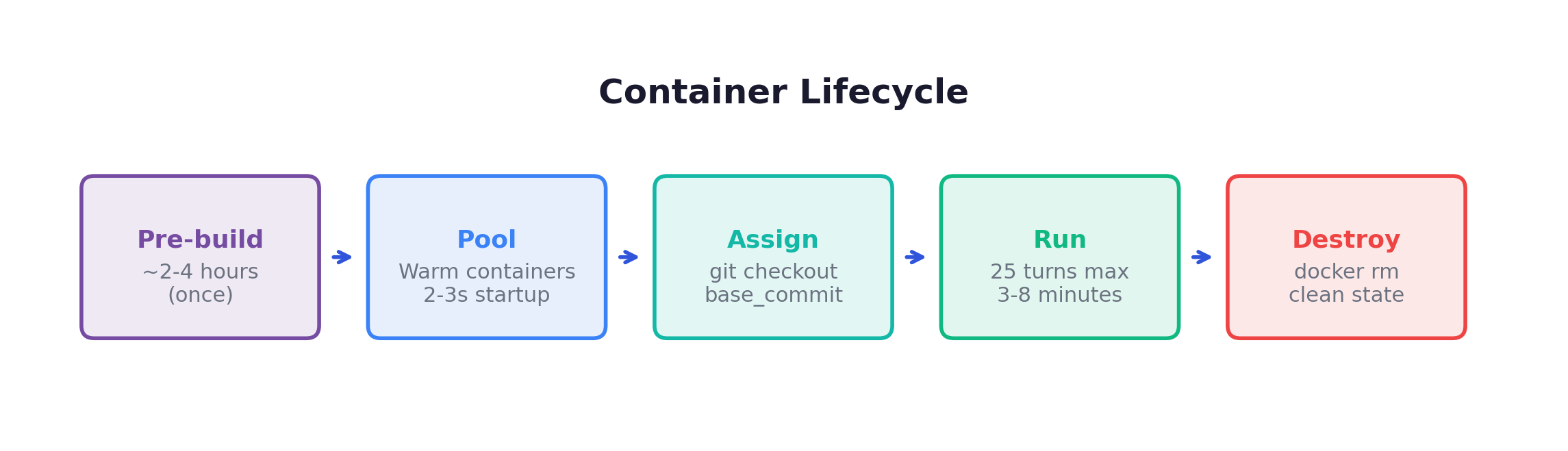
Container reuse optimization: If consecutive tasks come from the same repo, the worker resets the container (git checkout + git clean) instead of destroying and recreating it — saving 30-60 seconds per lifecycle.
The Agent Environment in Code
In Slime’s inverted design, the environment drives the loop by calling the rollout engine’s OpenAI-compatible API. Here’s the skeleton — the core loop that runs for each (task, rollout) pair:
       class AgentEnvironment:
    """Slime's inverted design: environment drives the loop via OpenAI API."""

    def __init__(self, worker_id, max_turns=50, timeout_seconds=600):
        self.worker_id = worker_id
        self.max_turns = max_turns
        self.timeout = timeout_seconds
        self.client = OpenAI(base_url="http://sgl-router:8000/v1")

    def collect_trajectory(self, task):
        """Main entry point: collect one trajectory."""
        start_time = time.time()

        # Step 1: Set up container
        container = DockerEnvironment(task["repo"], task["base_commit"])
        container.start()  # 2-3s with warm pool, 30-60s without

        # Step 2: Prepare conversation
        messages = [
            {"role": "system", "content": SYSTEM_PROMPT},
            {"role": "user", "content": task["issue_description"]},
        ]

        # Step 3: Agent interaction loop — environment calls rollout engine
        turns = []
        try:
            for turn_idx in range(self.max_turns):
                if time.time() - start_time > self.timeout:
                    break  # Hard timeout

                # Call rollout engine via OpenAI-compatible API
                response = self.client.chat.completions.create(
                    model="policy", messages=messages, temperature=0.7
                )
                assistant_msg = response.choices[0].message.content
                action = parse_action(assistant_msg)

                # Execute in container
                observation = container.execute_tool(action.tool, action.args)

                turns.append(TrajectoryTurn(
                    turn_index=turn_idx,
                    assistant_output=assistant_msg,
                    observation=observation,
                    tokens_generated=response.usage.completion_tokens,
                ))

                messages.append({"role": "assistant", "content": assistant_msg})
                messages.append({"role": "tool", "content": observation})

                if action.type == "submit":
                    break

            # Step 4: Run tests and compute reward
            test_results = container.run_tests(task["test_patch"])
            reward = 1.0 if test_results["all_passed"] else 0.0
        finally:
            container.stop()  # Always clean up

        # Step 5: Package trajectory
        return Trajectory(
            task_id=task["task_id"],
            system_prompt=SYSTEM_PROMPT,
            user_prompt=task["issue_description"],
            turns=turns,
            reward=reward,
            metadata={"worker_id": self.worker_id,
                      "elapsed_s": time.time() - start_time,
                      "num_turns": len(turns)},
        )
For GRPO with G=8, the Rollout Manager spawns 8 AgentEnvironment instances for each task, each calling collect_trajectory() independently. With 32 workers in the pool, 8 trajectories for one task complete in parallel in 3-8 minutes.
Why Inverted Design?
This pattern — environment drives the loop, policy is a service — might seem like a minor API choice, but it has deep architectural consequences that matter specifically for agentic RL.
Natural fit for async and variable-length episodes. In agentic tasks, one trajectory might finish in 3 turns while another takes 50; one tool call returns in 0.1 seconds while another compiles for 30 seconds. A traditional framework-driven sync loop would block the entire GPU cluster waiting for the slowest environment. With inverted design, each environment is an independent client — whoever needs the model’s next decision fires an HTTP request. The backend inference engine (SGLang/vLLM) applies continuous batching across these requests, keeping GPU utilization high regardless of how unevenly the environments progress.
Decoupled state management. SWE-bench environments are Docker containers with complex internal state — file systems, running processes, installed dependencies. If the RL framework had to track and synchronize thousands of container states, the orchestration logic would be fragile and error-prone. With inverted design, each environment manages its own lifecycle. The framework never touches container internals — it just serves inference requests and consumes finished trajectories from the data buffer.
CPU/GPU resource isolation. Environment execution (compiling code, running test suites, rendering web pages) is CPU- and memory-intensive. Model inference is GPU-intensive. The inverted design naturally separates these into a microservice topology: thousands of lightweight environment instances on cheap CPU nodes, calling a small cluster of GPU servers for inference. This is exactly what the Production Infrastructure section below describes.
Heterogeneous environment unification. Perhaps the most powerful consequence: inverted design lets fundamentally different environment types — code sandboxes, web browsers, mobile apps, terminal sessions — coexist in the same training loop without the framework knowing the difference. In a traditional framework-driven approach, the framework must parse each environment’s state representation (HTML DOM vs. terminal output vs. screenshot), dispatch the right action format, and handle type-specific edge cases (browser captchas, compilation timeouts, app crashes) — resulting in fragile, ever-growing orchestration code. With inverted design, the LLM’s chat API becomes a universal protocol: every environment, regardless of internal complexity, translates its current state into a text or multimodal prompt and calls the same endpoint. The framework sees only HTTP requests. This is what enables GLM-5’s Multi-Task Rollout Orchestrator to run coding, terminal, and search-agent tasks concurrently — each with independent rollout logic, all hitting the same inference cluster. (See the companion post on RL infrastructure for details.)
When is inverted design unnecessary? For math/reasoning RLVR (GRPO on GSM8K, AIME, etc.), the “environment” is just a stateless verifier that checks answers in milliseconds. There’s no multi-turn interaction, no container state, no variable-length episodes. A simple synchronous loop works perfectly — and adds no unnecessary complexity. Inverted design is specifically a response to the challenges in Section 1: stateful environments, multi-turn episodes, and heavy-tailed duration distributions.
Not all agentic frameworks use inverted design. Poolside’s Model Factory, for example, uses the traditional pattern: a framework-side Worker drives the loop, calling the code execution environment as a service. As their engineering blog describes: “the worker can simply invoke our code execution environment with a predefined set of inputs and collect the outputs. In some other settings, we may employ an agentic setup, allowing the worker to re-interact with the code execution environment across multiple iterations.” This works well for their use case — code execution is fundamentally a batch job (submit code → execute → return logs), and the worker can manage the interaction loop without the environment needing to take control. The tradeoff: the framework must understand the environment’s interaction patterns, which limits flexibility when adding new environment types. (For a detailed comparison of all three environment integration patterns, see the companion post on RL infrastructure.)
Production Infrastructure
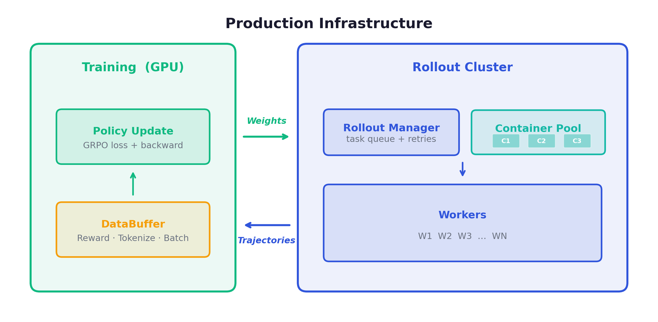
Rollout Manager: Maintains the task queue, assigns tasks to workers, handles failures and retries.
Worker Pool: 32-128+ workers, each handling one trajectory at a time. CPU-bound (container management), not GPU-bound.
Container Pool: Pre-warmed containers ready for immediate assignment.
Model Server: vLLM/SGLang instances serving the policy model. This is the GPU-intensive component. (For a deeper dive into how model serving, weight synchronization, and GPU orchestration work at scale across different frameworks, see RL Infrastructure for Large-Scale Agentic Training.)
Resource Budget
| Component | Resources | Notes |
|---|---|---|
| Training GPUs | 8× H100 80GB | Policy + reference model + GRPO |
| Rollout Inference | 4× H100 | vLLM for agent generation |
| Container Pool | 32-64 containers | ~4 GB RAM each, CPU nodes |
| Training Duration | ~3 days (3 epochs) | 500 SWE-Bench tasks, G=8 |
| Per-Trajectory | 2-10 minutes | Depends on task complexity |
The Long-Tail Problem
The defining operational challenge: trajectory durations follow a heavy-tailed distribution.
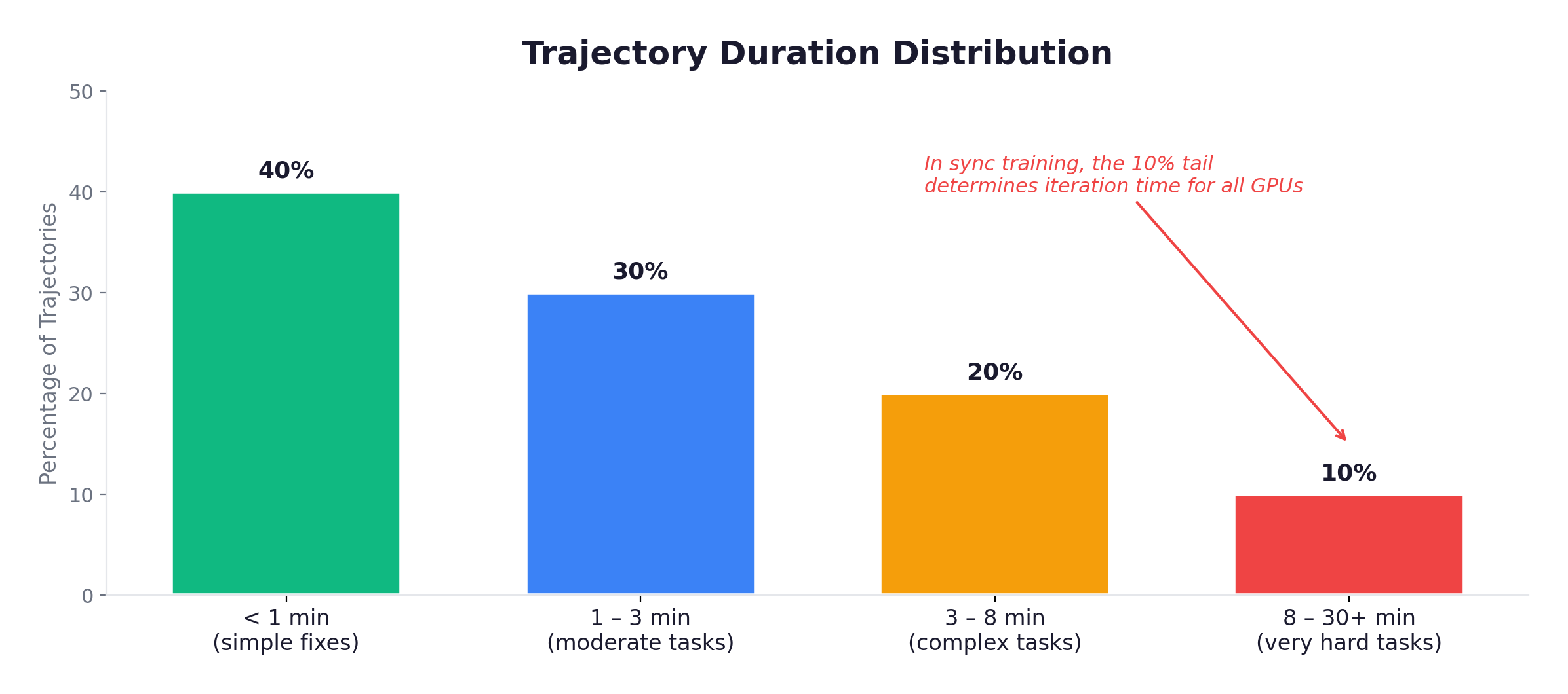
In synchronous training, the batch completes when the slowest trajectory finishes. If 63 out of 64 finish in 3 minutes but one takes 25 minutes, GPU utilization for the fast trajectories: 12%. This is why async training (APRIL), hard timeouts, and max-turn limits are essential.
Common Failure Modes
| Failure | Mitigation |
|---|---|
| Agent stuck in a loop | Max-turn limit + loop detection + custom_filter_fn |
| Container OOM | Per-container resource limits, memory monitoring |
| Network timeout to model server | Request timeout + retry |
| Zombie containers | Periodic cleanup, container TTL |
| Worker crash mid-trajectory | Heartbeat monitoring, auto-restart |
The most insidious failure is the loop: the agent tries a fix, it partially fails, it tries a slight variation, partially fails again, and repeats indefinitely. Without detection, this burns compute for zero training signal. Slime’s custom_filter_fn catches these: trajectories approaching max turns with zero reward are likely loops and should be discarded.
Async-specific failure modes. Asynchronous training introduces two additional categories of bad samples that synchronous setups don’t face:
Off-policy staleness. In async RL, long trajectories can become highly off-policy — they were started under a model version that has since been updated multiple times. GLM-5 handles this by logging the policy weight version used by the rollout engine at generation time. For each response, they record the sequence of model versions involved with . A sample is discarded if its oldest rollout version lags too far behind the current policy: , where is the current version and is a predefined threshold.
Environment crashes as noise. Coding-agent sandboxes are inherently unstable — containers OOM, test suites hang, network timeouts occur. These failures reflect environment instability, not model capability, and injecting them as negative reward would corrupt the training signal. GLM-5 records the failure reason for each sample and excludes those that fail due to environment collapse. For group-based methods like GRPO, removing failed samples can leave an incomplete group. They pad the group by repeating valid samples if the number of valid samples exceeds half of the group size; otherwise, the entire group is dropped.
6. The GRPO Algorithm in Detail
GRPO (Group Relative Policy Optimization) is the algorithm behind virtually every native agentic RL system. Understanding it in detail — not just the intuition, but the actual loss computation — is essential for reasoning about training behavior.
Core Idea: No Value Model, Just Comparison
Classical RL algorithms like PPO need a value function to estimate how good a state is, so they can compute advantages (how much better or worse an action was compared to expectation). Training this value function requires a separate neural network with its own forward/backward passes — for a 7B policy, that’s another ~84 GB of GPU memory.
GRPO’s insight: replace the value function with group comparison. Generate G trajectories for the same prompt, compare their rewards, and use the group statistics as the baseline:
If G=8 and 3 out of 8 trajectories succeed (reward=1.0), the successful ones get positive advantage, the failed ones get negative advantage. No learned baseline needed — the group is the baseline.
The Loss Function
The pseudocode is deceptively simple:
       def grpo_loss(log_probs_new, log_probs_old, advantages, loss_mask, ref_log_probs):
    # Importance ratio
    ratio = exp(log_probs_new - log_probs_old)

    # Clipped objective (prevents too-large updates)
    surr1 = ratio * advantages
    surr2 = clip(ratio, 1 - eps, 1 + eps) * advantages
    policy_loss = -min(surr1, surr2)

    # KL penalty (keeps policy close to reference model)
    kl_loss = beta * (log_probs_new - ref_log_probs)

    # Apply mask: only compute on assistant tokens
    loss = ((policy_loss + kl_loss) * loss_mask).sum() / loss_mask.sum()
    return loss
Three components:
-
Policy ratio
exp(log_new - log_old): how much more likely the current policy makes these tokens compared to the policy that generated them. Ratio > 1 means the current policy prefers these tokens more; < 1 means less. -
Clipping: prevents catastrophically large updates. If the ratio exceeds
[1-eps, 1+eps], the gradient is zeroed — the policy has already changed enough from this sample. -
KL penalty: prevents the policy from drifting too far from the reference model (the initial SFT checkpoint). Without this, the policy can degenerate into repetitive, reward-hacking behavior.
A Complete GRPO Training Step in PyTorch
Here’s the full implementation — advantage computation through gradient update — so you can see how the pieces fit together:
       import torch
import torch.nn.functional as F

def compute_group_advantages(rewards, group_size, clip_value=5.0):
    """
    Compute group-relative advantages.

    Args:
        rewards: (batch_size,) where batch_size = num_prompts * G
        group_size: G, number of trajectories per prompt
    Returns:
        advantages: (batch_size,) normalized within each group
    """
    G = group_size
    num_prompts = rewards.shape[0] // G

    # Reshape to (num_prompts, G)
    grouped = rewards.view(num_prompts, G)

    # Normalize within each group
    mean = grouped.mean(dim=1, keepdim=True)
    std = grouped.std(dim=1, keepdim=True).clamp(min=1e-8)
    advantages = (grouped - mean) / std

    # Clip extreme values (GRPO++)
    advantages = advantages.clamp(-clip_value, clip_value)
    return advantages.view(-1)


def grpo_training_step(model, ref_model, batch, optimizer,
                       group_size=8, clip_ratio=0.2, kl_coeff=0.01):
    """Complete GRPO training step."""
    input_ids = batch["input_ids"]           # (B, L)
    attention_mask = batch["attention_mask"]  # (B, L)
    loss_mask = batch["loss_mask"]            # (B, L) — 1 for assistant tokens
    old_log_probs = batch["old_log_probs"]   # (B, L)
    rewards = batch["rewards"]               # (B,)

    # Step 1: Group-relative advantages
    advantages = compute_group_advantages(rewards, group_size)

    # Step 2: Current policy forward pass
    logits = model(input_ids=input_ids, attention_mask=attention_mask).logits
    shift_logits = logits[:, :-1, :]
    shift_labels = input_ids[:, 1:]
    shift_mask = loss_mask[:, 1:]
    shift_old = old_log_probs[:, 1:]

    log_probs = F.log_softmax(shift_logits, dim=-1)
    token_log_probs = log_probs.gather(2, shift_labels.unsqueeze(2)).squeeze(2)

    # Step 3: Reference model log-probs (for KL)
    with torch.no_grad():
        ref_logits = ref_model(input_ids=input_ids,
                               attention_mask=attention_mask).logits[:, :-1, :]
        ref_log_probs = F.log_softmax(ref_logits, dim=-1)
        ref_token_log_probs = ref_log_probs.gather(
            2, shift_labels.unsqueeze(2)).squeeze(2)

    # Step 4: GRPO loss
    ratio = torch.exp(token_log_probs - shift_old)
    token_advantages = advantages.unsqueeze(1).expand_as(token_log_probs)

    surr1 = ratio * token_advantages
    surr2 = torch.clamp(ratio, 1 - clip_ratio, 1 + clip_ratio) * token_advantages
    policy_loss = -torch.min(surr1, surr2)

    kl_loss = kl_coeff * (token_log_probs - ref_token_log_probs)
    total_loss = ((policy_loss + kl_loss) * shift_mask).sum() / shift_mask.sum()

    # Step 5: Update
    optimizer.zero_grad()
    total_loss.backward()
    torch.nn.utils.clip_grad_norm_(model.parameters(), max_norm=1.0)
    optimizer.step()

    return {
        "loss": total_loss.item(),
        "mean_advantage": advantages.mean().item(),
        "mean_ratio": ratio.mean().item(),
        "kl": (token_log_probs - ref_token_log_probs).mean().item(),
    }
The key detail to notice: token_advantages is a scalar per trajectory, broadcast across all token positions. Every assistant token in a successful trajectory gets the same positive advantage; every token in a failed trajectory gets the same negative advantage. The loss mask ensures only assistant tokens receive gradients — the shift_mask.sum() normalization in the denominator means the loss is averaged over trainable tokens, not all tokens.
GRPO++ : Length Normalization
Standard GRPO has a bias: longer trajectories contain more tokens, so they contribute more to the total loss. Since successful trajectories on hard tasks tend to be longer (more turns of exploration), the model learns to generate verbose responses even on easy tasks — a phenomenon called length hacking.
GRPO++ adjusts rewards by trajectory length:
       adjusted_reward = reward * (target_length / actual_length) ** alpha
# alpha = 0.5, target_length = 2000 tokens
Short successful trajectories get amplified rewards, discouraging unnecessary verbosity. This is particularly important in agentic tasks where trajectory lengths vary from 500 to 50,000 tokens.
Advantage Estimation Methods Compared
| Method | Value Model? | Granularity | Variance | Cost |
|---|---|---|---|---|
| GRPO | No | Per-trajectory | Medium | Low |
| PPO/GAE | Yes | Per-step | Low | High (~84 GB) |
| RLOO | No | Per-trajectory | Medium | Low |
| iStar | No | Per-step | Low | Medium |
GRPO dominates for agentic RL because it’s cheap (no value model), effective (group comparison provides a good baseline), and simple (the implementation fits in ~50 lines of PyTorch).
7. From Single-Agent Training to Multi-Agent Deployment
The Train-Deploy Gap
Here’s a disconnect that bothered me when I first studied agentic RL: we train a single agent to solve tasks, but deploy it as part of a multi-agent system. In production, a coding agent might have a Lead that decomposes tasks, Experts that write code, and Reviewers that check work. During training? A single agent tries everything alone.
Shouldn’t we train the way we deploy?
The short answer: we should, but we mostly can’t yet. Multi-agent training is an active research frontier with promising but preliminary results.
Why Single-Agent Training Dominates
Search space explosion: A single agent’s trajectory already has an astronomical space of possible behaviors. Two interacting agents roughly doubles the dimensionality — exponentially more samples needed for convergence.
Credit assignment compounds: With one agent, GRPO’s coarse assignment (same advantage for all turns) works. With two agents, we need to determine which agent’s actions caused success. If the Lead delegated poorly but the Expert solved it anyway, the Lead gets undeserved credit.
Infrastructure cost multiplies: Multi-agent rollouts require multiple inference calls per step, coordinated container access, and more complex trajectory recording. The already-dominant rollout phase gets even longer.
“Train Single, Deploy Multi” — Why It Works
The same base model serves all roles, differentiated only by system prompt:
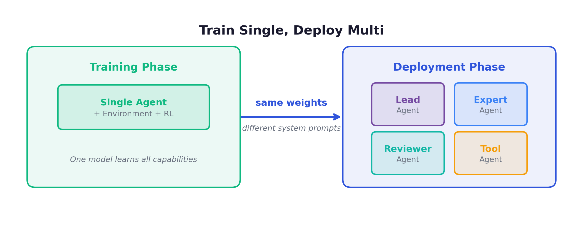
This works better than you might expect because the capabilities of a strong single agent naturally transfer to multi-agent roles:
| Single-Agent Capability | Multi-Agent Application |
|---|---|
| Tool use | Inter-agent communication |
| Step-by-step planning | Task delegation |
| Error recovery | Handling sub-agent failures |
| Context management | Working with delegated sub-tasks |
| Instruction following | Role adaptation via system prompt |
Three Approaches to Narrowing the Gap
Approach A: Diverse training prompts. Train with system prompts that simulate different roles — some rollouts use a “lead agent” prompt, some use an “expert” prompt, some use a “reviewer” prompt. The model learns role-adaptive behavior. Simplest approach, no infrastructure changes needed.
Approach B: Self-play. During rollout, the same model plays multiple roles in a simulated multi-agent interaction, with different system prompts. The trajectory captures the full team conversation. Reward is based on the team outcome. More expensive (3× inference calls per step) but produces more realistic training data.
Approach C: Sequential specialization. First train a strong base via single-agent RL. Then fine-tune role-specific variants — Lead, Expert, Reviewer — on role-appropriate trajectories. Creates specialized models from the same base.
The Research Frontier: True Multi-Agent RL
M-GRPO (Ant Group / Imperial College London): Decomposes team reward into per-agent contributions using Shapley values, then computes separate GRPO advantages for each role:
Multi-Agent Rollout example: Lead assigns “Fix the auth bug” → Expert1 searches, reads, edits → Expert2 runs tests, reports → Lead reviews, accepts. Team Reward: 1.0
| Role | Shapley Value | GRPO Advantage Formula |
|---|---|---|
| Lead | 0.3 | |
| Expert1 | 0.5 | |
| Expert2 | 0.2 |
Each role gets its own gradient signal. The Lead learns what makes delegation effective, independent of the Expert’s coding quality.
The challenge: exact Shapley computation evaluates all agent subsets — exponential. For 3 agents, that’s 8 evaluations. For 10 agents, over 1000. Here’s the exact computation:
       def shapley_values(agents, value_fn):
    """
    Exact Shapley values for each agent.

    phi_i = sum_{S ⊂ N\{i}} |S|!(|N|-|S|-1)!/|N|! × [v(S∪{i}) - v(S)]
    """
    n = len(agents)
    shapley = {agent: 0.0 for agent in agents}

    for agent in agents:
        others = set(agents) - {agent}
        for size in range(len(others) + 1):
            for subset in combinations(others, size):
                coalition = frozenset(subset)
                marginal = value_fn(coalition | {agent}) - value_fn(coalition)
                weight = factorial(size) * factorial(n - size - 1) / factorial(n)
                shapley[agent] += weight * marginal
    return shapley

# Example: 3-agent team solving a coding task
# value_fn simulates team performance:
#   Lead alone: 0.2 (can plan but not code)
#   Coder alone: 0.4 (can code but unguided)
#   Lead + Coder: 0.7 (guided coding)
#   All three: 1.0 (full team)

# Result: Lead=0.283, Coder=0.483, Reviewer=0.233
# → Coder contributes most, but Lead's coordination adds synergy
Monte Carlo approximation helps at scale — sample random agent orderings, compute marginal contributions — but adds noise to an already noisy RL signal.
SHARP (Shapley-based Hierarchical Attribution): Exploits the hierarchical structure of multi-agent systems. Instead of computing Shapley over all agents simultaneously:
- Level 1: Manager vs. workers-as-a-group (a cheap 2-player game). Manager’s Shapley value:
0.5 × (v_manager - v_empty) + 0.5 × (v_all - v_workers). - Level 2: Decompose the workers’ share among individual workers using standard Shapley within the worker group.
This reduces cost from to while preserving fairness properties.
Honest Assessment
What works now: Single-agent training + role-specific system prompts. This is the production standard.
What’s promising: M-GRPO with 2-3 agents. Self-play for generating realistic trajectories.
What doesn’t work yet: Training 5+ agents jointly. Learning emergent role specialization. Multi-agent training without 3-10× compute overhead.
Where the field is heading: Constitutional AI for defining role behaviors as rules. Modular RL with pluggable skill modules. Curriculum approaches starting single-agent and gradually introducing collaboration.
8. Reward Design: Beyond Binary
While binary reward (1.0 if tests pass, 0.0 otherwise) is the baseline that works, the reward function is one of the most important design decisions in agentic RL. Let’s survey the options.
Binary Reward
       def binary_reward(trajectory):
return 1.0 if trajectory.test_results["all_passed"] else 0.0Pros: Clear signal, no reward hacking, simple to implement. Cons: Extremely sparse — in early training, most trajectories get 0.0, providing no gradient signal beyond “don’t do this.”
Composite Reward
Weighted combination of multiple signals:
       def composite_reward(trajectory):
    test_pass = 1.0 if all_tests_pass else 0.0
    partial = passed_tests / total_tests        # Partial credit
    format_ok = 1.0 if valid_patch else 0.0     # Format compliance
    efficiency = max(0, 1.0 - turns / max_turns)  # Fewer turns = better

return 0.6 * test_pass + 0.2 * partial + 0.1 * format_ok + 0.1 * efficiencyPros: Denser signal, especially early in training. Cons: Weights require tuning, and components can be gamed (model optimizes for format compliance at the expense of correctness).
Staged Reward
Partial credit for progress milestones:
| Stage | Milestone | Reward |
|---|---|---|
| 0 | No meaningful action | 0.0 |
| 1 | Found the relevant file | 0.1 |
| 2 | Made a code change | 0.3 |
| 3 | Code compiles | 0.5 |
| 4 | Some tests pass | 0.7 |
| 5 | All tests pass | 1.0 |
Pros: Provides gradient signal even for trajectories that didn’t fully succeed — the model learns that finding the right file is better than random exploration. Cons: Stage detection adds implementation complexity, and intermediate stages can become local optima.
Length Penalty
GRPO++ applies a cosine-based length penalty:
       def length_penalized_reward(base_reward, num_tokens, target=2000, max_tokens=8000):
    if num_tokens <= target:
        return base_reward  # No penalty for concise solutions
    progress = (num_tokens - target) / (max_tokens - target)
    penalty = 0.5 * (1 + cos(pi * min(progress, 1.0)))
    return base_reward * penalty
Critical for agentic tasks where the model can learn to pad trajectories with unnecessary exploration to look like it’s “trying hard.”
Practical Recommendation
Start with binary reward. It’s the simplest and least likely to introduce reward hacking. If training stalls because the signal is too sparse (success rate stays near 0%), add staged rewards to provide gradient signal for partial progress. Add length penalty if the model starts generating excessively long trajectories. Composite rewards are useful for fine-tuning but require careful weight tuning.
9. Putting It All Together — Key Takeaways
After working through the full agentic RL training pipeline, a few themes emerge:
The Algorithm Is Settled, The Engineering Is Not
GRPO with binary reward is the algorithm that works. Every major framework uses it or a close variant. The research frontier is not about inventing new loss functions — it’s about making the training loop run faster, more reliably, and at larger scale.
Environments Are the Bottleneck
In math RLVR, generation is 80-90% of wall-clock time. In agentic RL, the environment adds another layer: container startup, tool execution, test suite running. The total rollout phase can be 95%+ of training time. Every optimization in the infrastructure — container pre-warming, async training, loop detection, over-provisioning — translates directly into faster experiments and more efficient research iteration. I covered these infrastructure challenges in depth in RL Infrastructure for Large-Scale Agentic Training, which complements this post’s focus on the training algorithm and data pipeline.
Loss Masking Is Subtle But Critical
The decision to train on all assistant tokens (while masking environment tokens) is conceptually simple but has deep implications. It means the model learns a unified strategy across all turns, with coarse credit assignment. More sophisticated masking strategies (action-only, progressive, turn-selective) exist but haven’t demonstrated clear advantages in practice.
Single-Agent Training Works for Multi-Agent Deployment
The “train single, deploy multi” paradigm is pragmatic and effective. A strong single agent naturally acquires capabilities (tool use, planning, error recovery) that transfer to multi-agent roles via system prompt adaptation. True multi-agent training (M-GRPO, SHARP) is the research frontier — promising but not yet production-ready.
The Numbers That Matter
| Parameter | Value | Notes |
|---|---|---|
| Model size | 7B-32B | Common range for open-weight RL agents |
| Group size | G = 4-8 | Balance signal quality vs. compute |
| Max turns (training) | 50 | Cap worst-case trajectory length; inference on long-horizon tasks (SWE-Bench Pro) can reach 100-300 |
| Trajectory time | 3-15 minutes | Dominated by multi-turn interaction |
| Training iteration | 10 min sync, 5 min async | |
| Full training run | ~17-34 hours | 3 epochs, 500 tasks |
| Target metric | SWE-Bench Verified | Resolve rate |
| Current SOTA (open-weight) | ~80.2% | MiniMax M2.5 |
References
RL Training Infrastructure
- Slime: Zhipu AI (THUDM) — Blog | GitHub
- MiniMax Forge — M1 Technical Report | M2.1 Post-Training Insights | M2.5 Release
- Poolside Model Factory — Blog series (6 parts)
- VERL: ByteDance — GitHub
- OpenRLHF — GitHub
Agentic RL Frameworks
- DeepSWE: Agentica / Together AI — Blog | GitHub
- SWE-RL: Meta FAIR — arXiv:2502.18449 | GitHub
- AgentRL: THUDM — arXiv:2510.04206 | GitHub
- Agent-R1: USTC — arXiv:2511.14460 | GitHub
- VerlTool: Tiger AI Lab — arXiv:2509.01055 | GitHub
Algorithms
- GRPO: DeepSeekMath — arXiv:2402.03300
- DeepSeek-R1 — arXiv:2501.12948
- DAPO — arXiv:2503.14476
- APRIL: AMD / CMU / LMSYS / UCLA — arXiv:2509.18521
- M-GRPO: Ant Group / Imperial College London — arXiv:2511.13288
- PPO — arXiv:1707.06347
Benchmarks
- SWE-Bench Verified — GitHub | 500 human-validated tasks