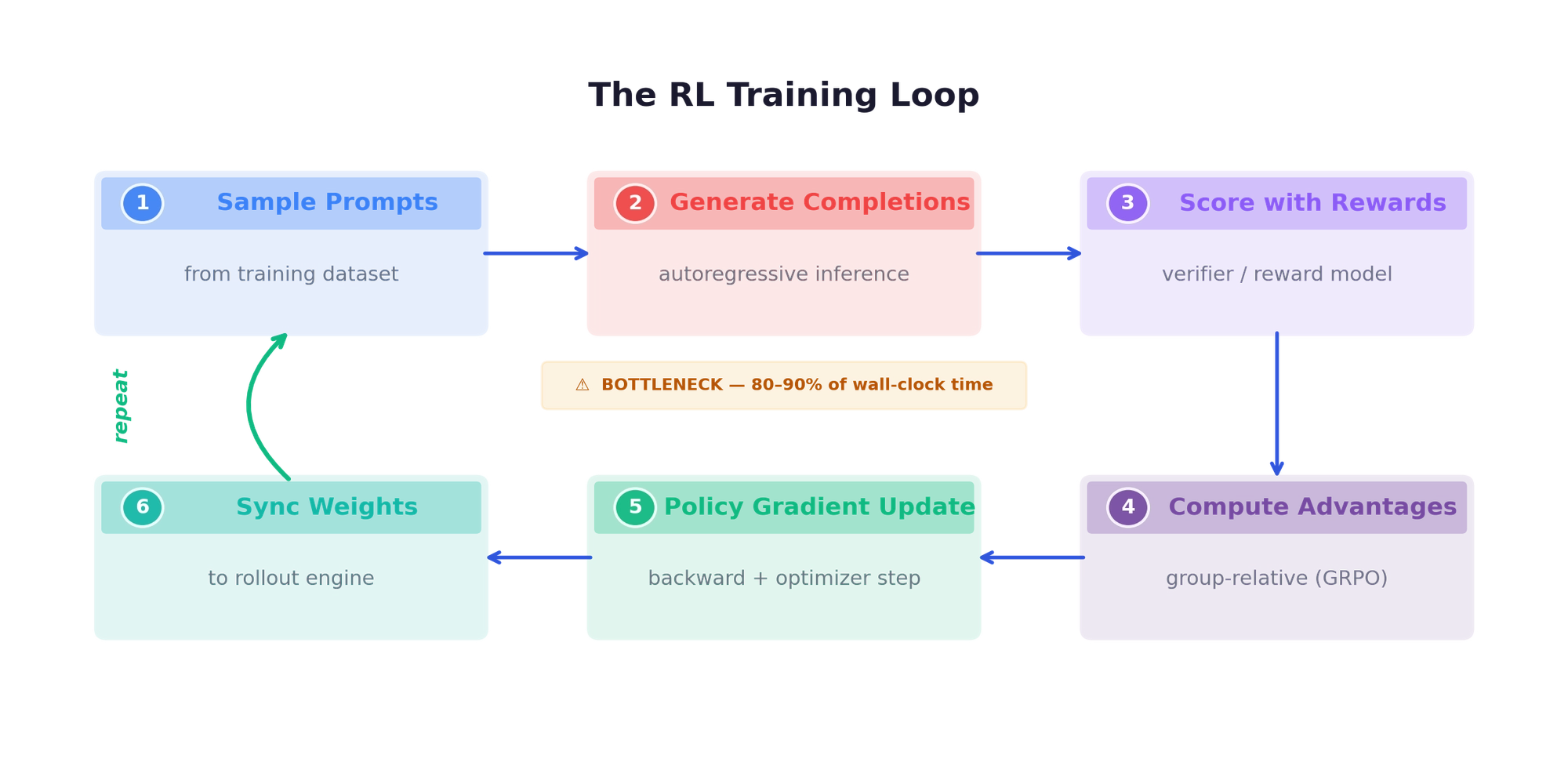
The recipe for training reasoning models is conceptually simple: generate solutions, verify correctness, update the policy. But at scale, 80–90% of training time is spent on sample generation alone. Infrastructure — not the loss function — is the primary constraint on experiment throughput.
I spent a few weeks digging into how the major RL training systems actually work — VERL, Slime, TorchForge, Poolside’s Model Factory, MiniMax Forge — reading their papers, blog posts, and source code. This post is a distillation of what I found. It’s organized around the questions I kept running into: where does the time go in an RL training loop? Why is weight sync so hard? What makes agentic RL architecturally different from math RLVR? And why do two implementations of “the same algorithm” produce different results?
Update (Feb 24, 2026): This post has been updated with production infrastructure details from the GLM-5 technical report, covering multi-task rollout orchestration, tail-latency optimization (PD disaggregation, FP8/MTP), DP-aware KV cache routing, and heartbeat-driven fault tolerance.
1. The Infrastructure Landscape at a Glance
The RLVR recipe is well-known by now: take a pre-trained LLM, generate candidate solutions for problems with verifiable answers, reward correct ones, update with policy gradients, repeat. What’s less discussed is that the infrastructure choices baked into this loop — how generation is parallelized, how weights are synchronized, whether training is sync or async — have as much impact on final model quality as the choice of algorithm.
A few observations that kept coming up during this survey:
- GRPO eliminates the critic model — and a big part of the motivation is that fitting a separate value network alongside the policy on limited GPUs is an infrastructure pain point. The algorithm was partly shaped by hardware constraints.
- DAPO’s dynamic sampling (dropping prompts where all completions are correct or all wrong) only works if the framework handles variable-sized batches. This is a non-trivial requirement.
- Two implementations of “the same algorithm” can produce wildly different results based on padding vs. packing, sync vs. async weight updates, and inference engine sampling behavior.
In other words, understanding the infrastructure isn’t really separable from understanding the algorithms.
The Core Numbers
The memory and time budgets that constrain everything:
| Model Size (params) | Weight Memory (bf16) | Training Memory (w/ Adam) | Min GPUs (H100) |
|---|---|---|---|
| 7B | ~14 GB | ~84 GB | 1-2 |
| 13B | ~26 GB | ~156 GB | 2-4 |
| 70B | ~140 GB | ~840 GB | 8-16 |
| 671B (MoE) | ~1.3 TB | ~7.8 TB | 64+ |
And the time breakdown that drives all the architectural decisions in this post:
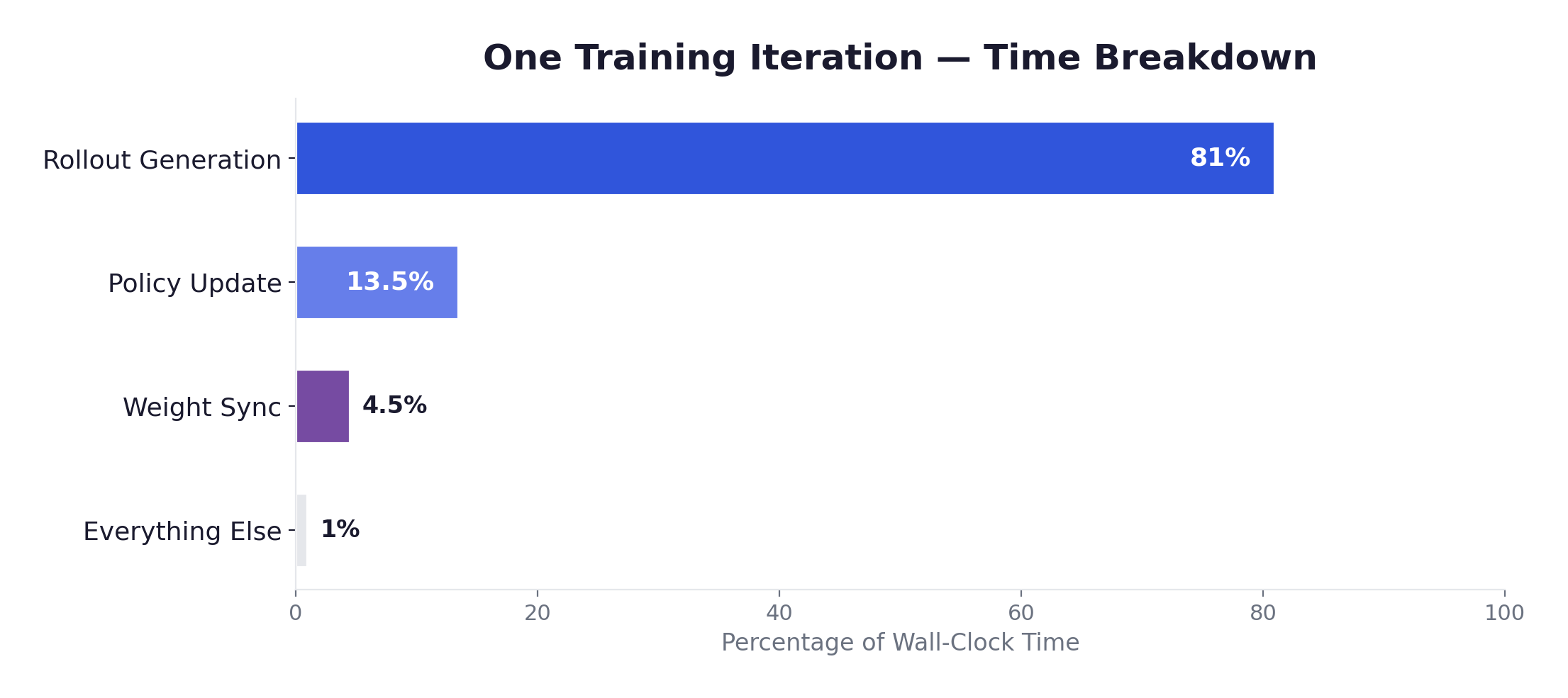
Generation is 80-90% of wall-clock time. This single fact shapes every design decision that follows.
Why is generation so slow? LLM inference is autoregressive — each output token requires a full forward pass, and each pass is memory-bandwidth-bound (not compute-bound) during the decode phase. For a 7B model generating a 2048-token response, decode alone takes ~4-8 seconds on a single A100. For a 70B model generating an 8192-token chain-of-thought response, it’s minutes per completion. With GRPO at G=8 and 128 prompts per batch, that’s 1024 completions per iteration. Even with vLLM/SGLang optimizations (paged attention, continuous batching, tensor parallelism), generation dominates by a factor of 5-10×.
This is qualitatively different from classical RL (Atari, MuJoCo), where environment steps are fast and policy updates are the bottleneck. In LLM-based RL, the roles are reversed — and the entire infrastructure stack is designed around this inversion.
2. Anatomy of an RL Training Loop
Five Model Roles
An RL training system for LLMs involves up to five distinct model roles, each with different hardware demands:
| Role | Purpose | Memory (7B, bf16) |
|---|---|---|
| Actor | Policy being trained (forward + backward) | ~84 GB (weights + optimizer + gradients) |
| Rollout | Fast autoregressive generation (vLLM/SGLang) | ~14 GB (weights) + ~40 GB (KV cache) |
| Reference | Frozen copy for KL divergence computation | ~14 GB (weights only) |
| Critic | Value function for GAE (PPO only) | ~84 GB (training memory) |
| Reward | Score completions (model or function-based) | Variable |
The iteration cycle: sample prompts → generate completions (the bottleneck) → score with rewards → compute advantages → policy gradient update → sync weights to rollout engine → repeat.
Algorithms and Their Infrastructure Footprints
The choice of algorithm directly determines the hardware requirements. The differences are larger than they might appear.
PPO needs all five roles — 4 models on GPU simultaneously:
| Role | Memory (7B, bf16) |
|---|---|
| Actor (training) | ~84 GB (weights + optimizer + gradients) |
| Critic (training) | ~84 GB (often same architecture as actor) |
| Reference (inference) | ~14 GB (weights only, bf16) |
| Rollout (inference) | ~14 GB (weights) + ~40 GB (KV cache) |
| Total | ~236 GB → 3-4 H100 GPUs minimum |
The common workaround: colocate actor and rollout on the same GPUs (they share weights, alternating between training and generation phases), colocate actor and reference (reference is just the initial weights, or the LoRA base). Even so, fitting a separate critic is often the breaking point — which is exactly why GRPO was designed to eliminate it.
GRPO drops the critic (~84 GB saved) and replaces GAE with group-relative advantage: generate G completions per prompt (typically G=4-16), normalize rewards within each group. The tradeoff shifts from memory to compute: with G=8 and 128 prompts per batch, that’s 1024 completions per iteration. The inference engine needs to handle this efficiently — prefix sharing (KV cache reuse across the G completions sharing the same prompt) becomes essential, and SGLang’s StringRadixTrie is specifically designed for this.
DAPO builds on GRPO with four innovations that each carry infrastructure implications:
- Clip-Higher: asymmetric upper/lower clip bounds to promote diversity. Minimal infra impact — just a different clip value.
- Dynamic Sampling: filter out prompts where all completions are correct or all wrong (zero advantage). This is the hard one — batch sizes become variable after filtering, and the training framework must handle it cleanly.
- Token-Level Policy Gradient Loss: normalize by total token count, not sequence count. Interacts non-trivially with sequence packing.
- Overlong Reward Shaping: soft penalty for responses exceeding 16K tokens, with a 4K grace buffer. The KV cache must accommodate 20K-token sequences.
REINFORCE++ has the simplest generation pattern — one completion per prompt — but higher variance, potentially requiring more training iterations to converge. RLOO (Leave-One-Out) uses other samples in the batch as baselines, similar to GRPO’s multi-sample approach but with different advantage computation.
The Fundamental Tension
Training and inference compete for the same GPU memory, but need very different things:
| Workload | Memory (7B) |
|---|---|
| Training | weights (bf16) + optimizer (fp32) + gradients + activations = ~84 GB |
| Inference | weights (bf16) + KV cache = ~54 GB @ batch 64 |
| Combined | ~138 GB, but an H100 has only 80 GB |
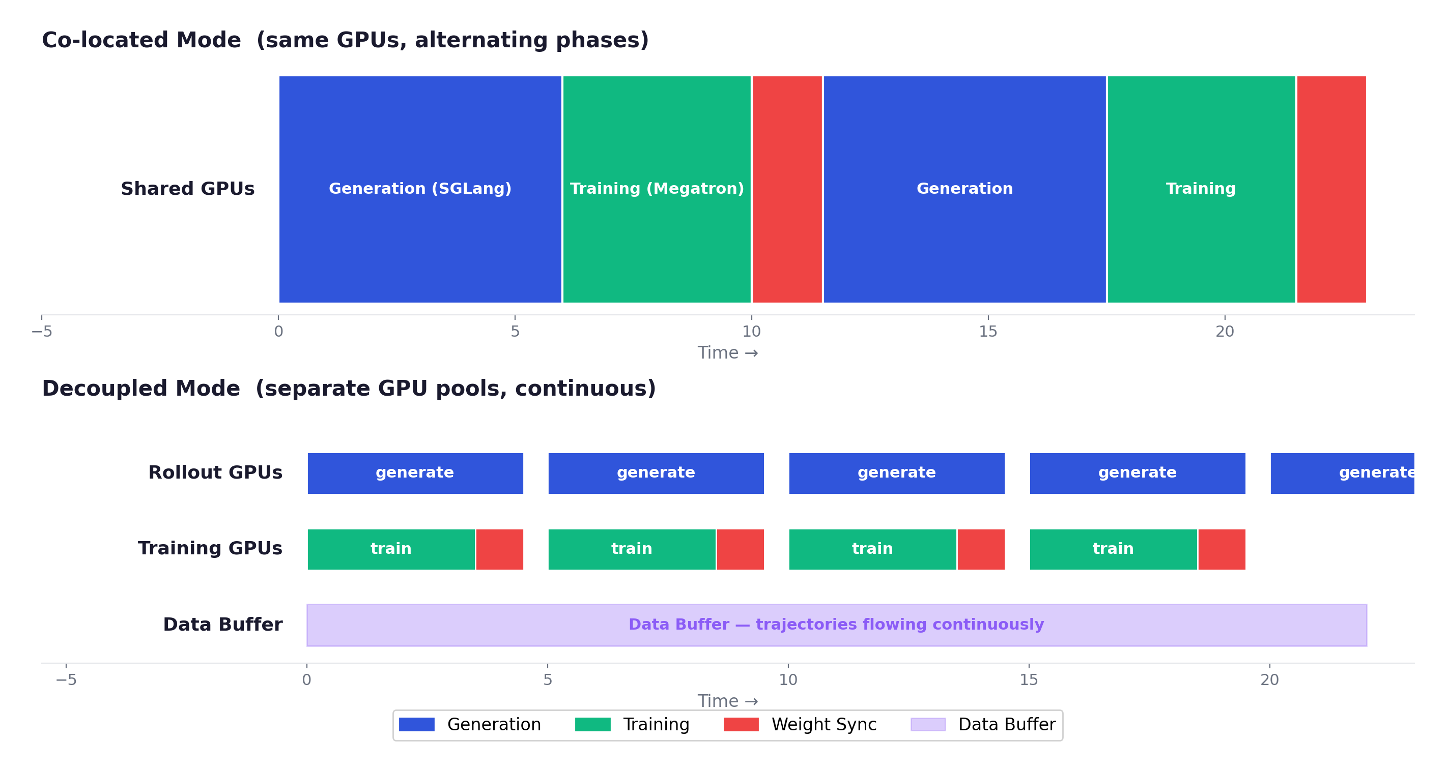
This forces a choice between colocated (share GPUs, alternate phases, no weight transfer needed but GPUs idle during the other phase) and disaggregated (separate GPU pools, both run optimally, but weight sync becomes a real problem). Every framework takes a position on this spectrum, and the right answer depends on model size, hardware availability, and whether generation or training dominates the iteration time.
A quick back-of-envelope for a 7B model with GRPO (G=8, 128 prompts):
| Phase | Setup | Time |
|---|---|---|
| Generation | 1024 completions × 2048 tokens, vLLM/SGLang, 2 GPUs (TP=2) | ~60–120s |
| Training | forward + backward + optimizer, 1024 samples, FSDP, 2 GPUs | ~15s |
| Weight Sync | depends on mechanism (see Chapter 6) | 7–60s |
| Total | 75–180s (generation = 70–90%) |
At 70B, everything scales up: generation takes 5-10× longer (the KV cache alone needs ~80 GB at reasonable batch sizes), training takes 5-8× longer, and weight sync must move 10× more data. The generation-dominance only gets more extreme.
Training-Inference Consistency
A subtler but equally important tension: the tokens produced during rollout generation must match the probabilities computed during training. This sounds obvious, but in practice the training engine (Megatron, FSDP + PyTorch) and the inference engine (vLLM, SGLang) are entirely different codebases with different numerical implementations. Several sources of inconsistency can creep in:
Numerical precision mismatches. Training typically runs in bf16/fp16 mixed precision with certain layers (loss computation, optimizer states) in fp32. Inference engines may use different precision for the same layers. MiniMax discovered this the hard way during M1 training: when migrating from a dense model to their MoE architecture, RL reward stopped improving entirely. After logging and comparing the training-time and inference-time token probabilities, they found that the correlation between training and inference log-probs was much lower than expected — with telltale “piecewise horizontal segments” in the correlation plots indicating quantization artifacts. Layer-by-layer debugging traced the root cause to the LM head (prediction layer): its high-magnitude activations amplified precision differences between the two engines. Restoring the LM head to FP32 brought the correlation from ~0.9x to ~0.99x, and training resumed making progress. This finding — that a seemingly small precision difference can completely stall RL training — is one of the more striking practical lessons in this space.
Sampling behavior differences. Different inference engines implement top-p, top-k, temperature, and repetition penalties differently. Even identical sampling parameters can produce different token distributions due to floating-point ordering in the softmax.
Tokenization and special token handling. Padding strategies, BOS/EOS token insertion, and chat template application may differ between training preprocessing and inference generation.
Why this matters specifically for RL: In supervised learning, small numerical differences between forward passes are tolerable — the loss landscape is smooth and gradients point in roughly the right direction regardless. But in RL with importance sampling (PPO, CISPO, GRPO), the algorithm computes the ratio between the current policy’s probability and the rollout policy’s probability for each token. If the probabilities computed during training systematically differ from those computed during inference (when rollouts were generated), these ratios are corrupted: the clipping mechanism clips the wrong tokens, gradient signals are distorted, and learning stalls. The model receives misleading training signals because it cannot accurately assess which actions improved or worsened outcomes. This is qualitatively different from the staleness problem (where probabilities differ because the policy changed) — here the probabilities differ because the computation differs, even for the same weights and inputs.
How frameworks address this:
- Slime uses the same SGLang server for both rollout generation and log-prob scoring, with an OpenAI-compatible API. One explicit design goal is “preventing discrepancies between the model’s performance during training and its metrics when deployed.”
- MiniMax Forge ensures training and inference are fully decoupled but token-consistent: the inference engine persists all logs during agent execution, and the Data Coordinator extracts trajectories with exact token sequences for training. The FP32 LM head fix is now standard practice for their MoE models.
- VERL uses the same model weights in-process (3D-HybridEngine reshards between training and inference parallelism layouts on the same GPUs), which reduces — though doesn’t eliminate — the risk of numerical divergence.
- OpenRLHF explicitly separates generation (vLLM) from scoring (HuggingFace forward pass), accepting the risk of minor inconsistency in exchange for simpler engineering.
The general lesson: for dense models at moderate scales, small precision differences are often tolerable. But for MoE models — where sparse routing can amplify numerical differences — and for long agentic trajectories — where small per-token errors compound over thousands of tokens — training-inference consistency becomes a first-order concern that can mean the difference between a training run that works and one that doesn’t.
3. Environments and Sandboxes
Four Tiers of Complexity
As we move from math RLVR toward agentic RL, environments become the other major infrastructure challenge:
Tier 1: Stateless Verifiers (milliseconds). Math answer checking, format compliance. CPU-only, trivially parallelizable. Not interesting from an infrastructure perspective.
Tier 2: Code Execution Sandboxes (seconds to minutes). Isolated containers, dependency management, test suite execution. This is where infrastructure starts to matter.
Tier 3: Interactive Tool Environments (variable). Web browsing, API calling, file manipulation. Stateful, persist across multiple model interactions.
Tier 4: Full Agent Environments (minutes to hours). SWE-bench style tasks: clone repo, understand codebase, write patch, run tests. Long-running, sometimes needing GPU access for sub-tasks.
Poolside’s RLCEF: A Reference Architecture
Poolside’s code execution environment is probably the most sophisticated publicly documented system for RL environment infrastructure. Worth studying in detail.
Saucer is their custom gRPC service for repository management: 800,000+ repositories indexed with Git packfile format and custom indexing for random access at any revision. A Kafka-backed (Redpanda) ingestion queue ensures reproducible processing.
OCI container isolation gives each repository its own image with all dependencies pre-installed. The key design choice: OverlayFS layering — a base image per repository plus thin delta layers per revision, avoiding quadratic storage growth. The system can spin up a container for any repository at any revision in seconds.
Building 800K repositories is itself a massive challenge. Poolside uses language-aware heuristic detection (Rust → Cargo, Python → pyproject.toml) for most languages, but C/C++ is handled by AI agents trained to understand READMEs and debug build failures. This is a notable self-improvement loop: Factory-trained agents now help build containers for complex C++ projects.
The Task Engine orchestrates millions of concurrent code executions for online RL. It exposes a session-based API — start session, modify filesystem, execute tests, get results — and supports developer-like async patterns where models submit new requests before receiving prior outcomes. Intelligent request routing co-locates repo revisions on the same server to share OverlayFS layers, minimizing container startup overhead.
”We now have an agent that was trained in the Factory working to improve the Factory.” — Poolside engineering team
This recursive self-improvement pattern is one of the most interesting aspects of their system: the same agents being trained by the infrastructure are also being used to extend the infrastructure’s capabilities.
MiniMax’s Approach
MiniMax takes a different angle — prioritizing breadth and speed:
- 5,000+ isolated environments launched within 10 seconds
- Concurrent operation of tens of thousands of environments
- 10+ programming languages (JS, TS, Python, Java, Go, C++, Kotlin, Rust, etc.)
- 100,000+ training environments sourced from real GitHub repositories with Issues, code, and test cases
- Kubernetes-based with storage-optimized instances for container image caching
Their M2.1 post details the environment construction pipeline: they filter GitHub PRs that were eventually merged and have relevant test cases, then build a runnable Docker environment for each PR — a non-trivial process where agents iteratively build environments with sandbox tools (and expert knowledge is still required for some languages). For bug-fix tasks, the system extracts F2P (Fail-to-Pass) and P2P (Pass-to-Pass) test cases — P2P tests being particularly important to ensure fixes don’t introduce new regressions. The result: 10,000+ runnable PRs across 10+ languages, with 140,000+ variable tasks generated through transformations like injecting additional bugs, merging commits, and converting bug-fix tasks into test-writing tasks.
The Long-Tail Problem
The defining infrastructure challenge of agentic RL: episode lengths follow a heavy-tailed distribution.
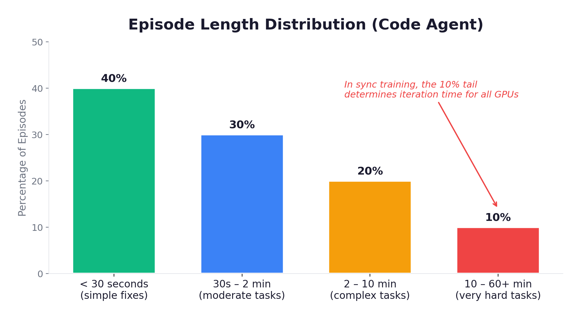
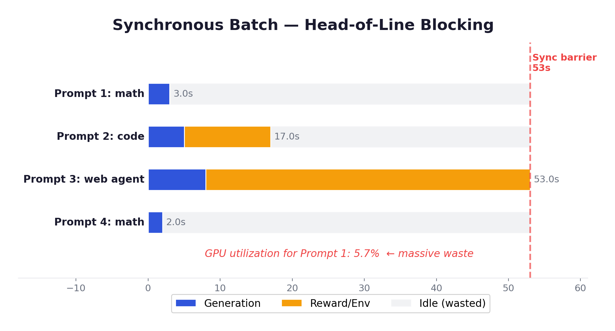
With synchronous training, the entire batch waits for the slowest episode. That 10% tail determines iteration time, while 40% of GPUs sit idle. The utilization math is brutal:
This is the problem that drove the entire field toward asynchronous training (Chapter 4).
Three approaches to this problem in current frameworks:
APRIL (Active Partial Rollouts) — integrated into Slime. The idea: over-provision rollout requests beyond what the training batch needs. As responses complete, they’re added to the training buffer. Once enough are ready, remaining in-progress generations are terminated and their partial trajectories recycled for continuation in future steps. Up to 44% throughput improvement, with up to 8% higher final accuracy (because the training buffer is biased toward completed episodes, which tend to be the more informative ones).
Request-Level Async — VERL AgentLoop, Slime. Each conversation progresses independently with no batch barriers. Fast episodes complete and free resources immediately, new episodes start as resources become available. This makes the straggler problem manageable without discarding data.
Partial Rollout Checkpointing — SkyRL and others. Pause long episodes, save their state, resume in a future iteration with updated weights. Prevents any single episode from blocking progress indefinitely, at the cost of some staleness in the resumed trajectories.
Environment Integration Patterns
Three patterns have emerged, each with a different philosophy about where the boundary between “framework” and “environment” should sit:
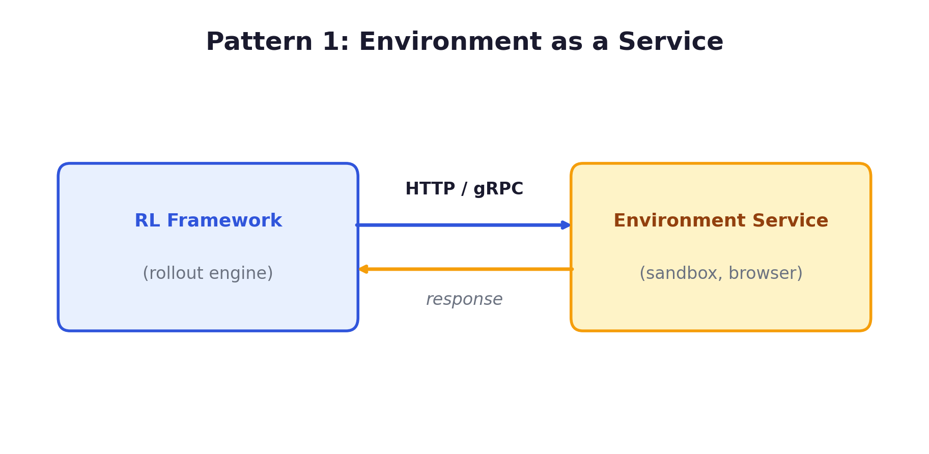
Pattern 1: Environment as a Service (Slime, VERL AgentLoop, Poolside). Environment and inference engine run as separate HTTP/gRPC services, communicating over the network rather than in-process. Clean separation — each component can be scaled independently. Within this pattern, the control flow can go either direction: in VERL AgentLoop and Poolside, the framework orchestrates the loop (calling the environment service for tool execution, calling the inference engine for generation); in Slime, the environment drives the loop — it calls the rollout engine’s OpenAI-compatible API for generation, executes tools locally, and produces trajectories that the training engine consumes from a data buffer. This inversion is detailed in Chapter 5.
Pattern 2: Gym-Style API (OpenEnv, TorchForge). The environment exposes step(), reset(), state() methods in-process:
       env = CodeExecutionEnv(repo="user/project", revision="abc123")
obs = env.reset()
for turn in range(max_turns):
    action = model.generate(obs)
    obs, reward, done, info = env.step(action)
    if done:
        break
Familiar to RL practitioners, composable, testable. OpenEnv (Meta + Hugging Face) is pushing this as a standard across the ecosystem.
Pattern 3: Agent Scaffold Redirect (MiniMax Forge). The agent’s API base URL is redirected to the RL framework’s inference engine during training. The agent runs completely unmodified — it doesn’t even know it’s being trained. This is the most radical approach: it works even for black-box binary executables where there’s no source code access. MiniMax’s Data Coordinator then extracts sub-agent trajectories from execution logs for the policy gradient computation.
4. Synchronous vs. Asynchronous Training
The Architecture Spectrum
The choice between sync and async training is one of the most consequential architectural decisions, and the field has converged on a clear spectrum.
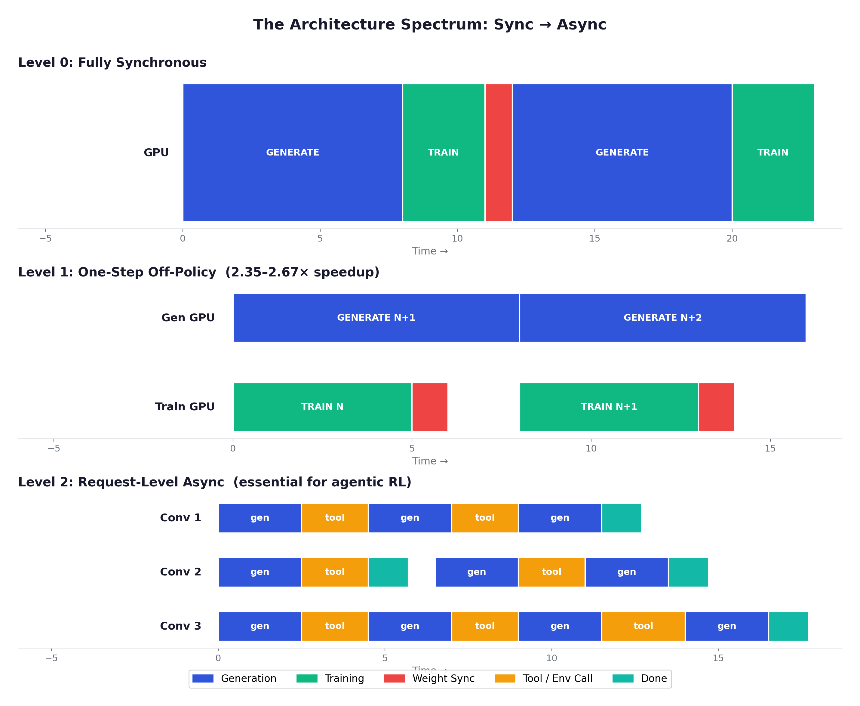
Level 0: Fully Synchronous. Generate all → Score all → Train → Sync weights → Repeat. Deterministic and easy to debug. But suffers from head-of-line blocking — every GPU waits for the slowest sample. Acceptable for math RLVR with uniform episode lengths.
Level 1: One-Step Off-Policy. Overlap current training with next batch’s generation. Rollout uses weights from the previous step. VERL reports 2.35x-2.67x improvement training Qwen2.5-7B on 128 GPUs with this approach. One step of staleness has minimal impact on training dynamics — the clipped objective naturally handles small distributional shifts.
Level 2: Request-Level Async. Each conversation progresses independently. No batch barriers. This is what makes agentic RL tractable. Without it, one conversation needing a 5-minute tool call blocks the entire batch.
Implementation: VERL uses AgentLoopBase (a per-conversation state machine); Slime uses native asyncio with an /abort_request endpoint for mid-generation interruption.
Level 3: Fully Asynchronous. Generation and training proceed independently on separate GPU pools. AReaL reports 2.77x speedup vs synchronous, but samples may be 2+ steps stale.
Engine Mode vs. Server Mode
A distinction that turned out to be more fundamental than I initially expected.
Engine mode — inference runs as an in-process library call:
       # Engine mode: everything blocks until all prompts complete
with torch.no_grad():
    outputs = vllm_engine.generate(prompts, sampling_params)
# Can't do anything until ALL prompts finish generating
All requests must complete before control returns. This makes multi-turn interaction essentially infeasible — if one conversation needs a 5-minute tool call, every other conversation blocks waiting.
Server mode — inference runs as a separate HTTP/RPC service:
       # Server mode: each request is independent
async def generate(prompt):
    response = await http_client.post(
        "http://sglang-server:8000/v1/completions",
        json={"prompt": prompt, "max_tokens": 4096}
    )
    return response.json()
Each request progresses independently. Dynamic batching. True request-level concurrency. The trade-off: network overhead, and weight sync requires an explicit mechanism since memory is no longer shared.
The trajectory here is clear: VERL v0.7 switched to server mode as default. Slime has always used server mode (even in co-located mode, Megatron and SGLang are separate processes). TorchForge uses Monarch services. Engine mode remains useful for simple single-turn RLVR on single nodes, but anything multi-turn or agentic requires server mode.
The Staleness Question
Async training introduces off-policy bias. The mechanics:
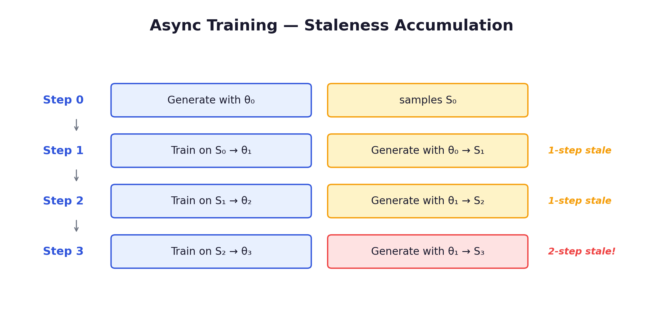
If the policy changes significantly between steps, stale samples have different probability distributions than the current policy. The importance sampling ratio π_θ(a|s) / π_θ_old(a|s) diverges, leading to high-variance updates or outright divergence.
How frameworks handle this:
| Framework | Staleness Correction | Tolerance |
|---|---|---|
| AReaL | Staleness-aware PPO + adjusted clipping | Full version tracking |
| VERL | Checkpoint Engine with version control | Recommends ≤1 step |
| Slime | Token-level importance sampling | On-policy default, IS correction available |
| PrimeRL | Cross-datacenter tolerance | Acknowledges 2+ steps |
| TorchForge | Weight version tracking in replay buffer | Configurable |
| GLM-5 | Rollout log-probs as direct proxy + double-sided clipping | Approximate; tokens outside hard-masked |
Staleness hurts most when: the policy changes rapidly (early training, high LR), rewards are sparse (most completions get 0; rare successes drive learning), and the action space is large (LLMs: exponentially large token space). It hurts least near convergence with dense rewards and small learning rates.
In practice, one-step staleness is almost always fine — the clipped surrogate in PPO/GRPO was literally designed to handle small distributional shifts. Fully async (2+ steps) requires more care. AReaL’s approach — tracking exact policy versions and adjusting clipping bounds based on staleness — is the most rigorous solution, achieving 2.77× speedup without training instability.
Turning staleness into an asset: cross-policy sampling. The discussion above treats staleness purely as a cost to be mitigated. AgentRL (THUDM / Z.AI) flips this perspective: stale model versions aren’t noise to be discarded — they’re a source of exploration diversity. In multi-turn agentic RL, model exploration typically declines over training as the policy converges, a problem that is more severe than in single-turn settings due to the larger state space. AgentRL’s cross-policy sampling strategy addresses this by maintaining a pool of models — the current policy plus earlier checkpoint versions (kept as “stale engines” that update parameters less frequently). At each step of a trajectory, the action is generated by a model randomly drawn from this pool rather than always from the current policy. This is distinct from GRPO’s multi-sample approach, which generates multiple complete trajectories per prompt using the same policy. Cross-policy sampling operates within a single trajectory, mixing actions from different model versions across turns. The result: trajectories explore paths that no single model version would discover alone, increasing the diversity of the training data. Ablation studies show clear gains in open-ended environments (e.g., knowledge graph navigation) where exploration collapse is most acute. The insight is worth noting for infrastructure design: frameworks that track and retain historical policy checkpoints for staleness correction (AReaL, VERL) could potentially reuse them as exploration engines — a dual-purpose use of infrastructure that’s already in place.
5. Slime’s Inverted Design
Slime is the framework I found most architecturally interesting. Developed by Tsinghua (THUDM) and Z.AI (formerly Zhipu AI), it’s the production RL infrastructure behind the GLM model family from GLM-4.5 through GLM-5. GLM-4.5 (355B/32B MoE) achieved 70.1% on TAU-Bench, 91.0% on AIME 2024, and 64.2% on SWE-bench Verified.
[2026-02 Update] Slime has since been used to train GLM-5 (744B total / 40B active MoE, 256 routed experts + 1 shared expert, 78 layers). GLM-5 achieved 77.8% on SWE-bench Verified and 75.9% on BrowseComp (with context management; 62.0% standard). The model was trained entirely on Huawei Ascend chips using MindSpore — making it the first frontier-scale MoE model fully trained on non-NVIDIA hardware, while the Slime framework itself remains hardware-agnostic (validated on both NVIDIA H100 and AMD MI300X). Slime is described in the GLM-5 release as “a novel asynchronous RL infrastructure that substantially improves training throughput and efficiency, enabling more fine-grained post-training iterations.” The technical report details Slime’s production extensions including multi-task rollout orchestration, tail-latency optimization, and DP-aware KV cache routing.
The Core Insight
Traditional RL frameworks try to control the environment interaction loop:
       # Traditional: framework must understand every environment type
class TraditionalFramework:
    def rollout(self, prompt):
        response = self.generate(prompt)
        tool_result = self.call_tool(response)     # framework manages tool calls
        response2 = self.generate(prompt + tool_result)
        return self.compute_reward(response2)
Every new environment type — code sandbox, web browser, file system, multi-turn dialogue — requires modifying the framework’s core rollout logic. The result is bloated, brittle code that covers only a fraction of real-world needs.
Slime inverts this. The environment drives the loop, not the framework:
       # Slime: environment controls the loop via standard OpenAI API
class AgentEnvironment:
    def __init__(self):
        self.client = OpenAI(base_url="http://sgl-router:8000/v1")

    def run_episode(self, task):
        messages = [{"role": "user", "content": task}]
        for turn in range(max_turns):
            response = self.client.chat.completions.create(
                model="policy", messages=messages,
            )
            action = response.choices[0].message.content
            if needs_tool_call(action):
                tool_result = self.execute_tool(action)
                messages.append({"role": "assistant", "content": action})
                messages.append({"role": "user", "content": tool_result})
            else:
                return self.compute_reward(messages)
The environment doesn’t know it’s talking to a training system. It uses the same OpenAI-compatible API it would use in production. This gives three properties that are hard to get any other way:
- Zero environment modification — any existing agent that calls an OpenAI API works with Slime during training, unmodified.
- Training-deployment consistency — same API in both contexts eliminates a class of subtle behavioral differences.
- Lightweight framework — Slime doesn’t need to understand environments; it just serves inference and consumes trajectories.
Why This Inversion Matters
The three properties above are real but somewhat abstract. To understand why Slime’s design is a structural advantage — not just an API preference — it helps to see what goes wrong at scale when the framework drives the loop, and how inversion resolves each failure mode.
The traditional approach breaks down in five ways
1. Variable-length episodes cause head-of-line blocking. In agentic RL, one trajectory might finish in 3 turns while another takes 50; one tool call returns in 100ms while another compiles code for 5 minutes. When the framework runs a synchronous for loop over all environments, the entire GPU cluster idles waiting for the slowest one. The utilization math is brutal — Chapter 3 shows how 40% of GPUs can sit idle in synchronous batches. Inverted design eliminates this: each environment is an independent HTTP client running at its own pace. The inference engine applies continuous batching across incoming requests, maintaining high GPU utilization regardless of how unevenly environments progress.
2. Stateful environments are expensive to manage externally. SWE-bench environments are Docker containers with complex internal state — file systems, running processes, installed dependencies, network configurations. If the framework orchestrates these environments, it must track and synchronize thousands of container states, handle environment-specific exceptions (compilation timeouts, test suite hangs, OOM kills), and implement recovery logic for each failure mode. This is fragile and error-prone. With inverted design, each environment manages its own lifecycle — the container handles its own state transitions, exception recovery, and cleanup. The framework never touches container internals; it just serves inference and consumes trajectories from the data buffer.
3. Heterogeneous environments can’t be unified — every new type requires framework changes. This is the most insidious scaling problem. In a framework-driven approach, the rollout logic must know how to parse each environment’s state representation — terminal output for code sandboxes, HTML DOM or screenshots for browsers, accessibility trees for mobile apps — and must dispatch the right action format for each. As environment types multiply, the framework accumulates if-else branches, type-specific middleware, and custom exception handlers. The codebase grows with every new use case.
Inverted design eliminates this entirely. The LLM’s chat API becomes a universal protocol: every environment, regardless of internal complexity, translates its current state into a text or multimodal prompt and calls the same OpenAI-compatible endpoint. The framework sees only HTTP requests — it cannot distinguish whether the caller is a Docker container compiling Rust, a headless browser navigating a website, or a mobile emulator tapping through an app. New environment types require zero framework changes.
This is what enables GLM-5’s Multi-Task Rollout Orchestrator to run coding, terminal, and search-agent tasks concurrently — each with independent rollout logic registered as a microservice, all hitting the same inference cluster.
4. Multi-agent and human-in-the-loop are awkward to retrofit. If the environment involves multiple agents (one writes code, another reviews it) or requires human approval at certain steps, a framework-driven loop must handle control-flow handoffs between different decision-makers. This quickly becomes a complex state machine. In the inverted model, the environment is the natural orchestration point — it calls whichever model (or waits for whichever human input) is needed at each step, using the same API for all of them.
5. CPU and GPU workloads compete for resources. Environment execution (compiling, running tests, rendering pages) is CPU- and memory-intensive. Model inference is GPU-intensive. A framework that drives both must either colocate them (wasting GPU memory on environment overhead) or build custom scheduling to alternate. Inverted design naturally separates these into a microservice topology: thousands of lightweight environment instances on cheap CPU nodes, calling a small cluster of expensive GPU servers through the network. Each resource pool scales independently.
Contrast: when traditional Pattern 1 works fine
Not all agentic systems need this inversion. Poolside’s Model Factory uses the traditional pattern — a framework-side Worker drives the loop, calling the code execution environment as a passive service. As their engineering blog describes:
“the worker can simply invoke our code execution environment with a predefined set of inputs and collect the outputs. In some other settings, we may employ an agentic setup, allowing the worker to re-interact with the code execution environment across multiple iterations.”
This works for Poolside because their primary interaction is code execution — a batch job with clear boundaries (submit code → execute → return logs). The environment doesn’t need to take initiative or manage complex state transitions between calls. The framework can handle the simple request-response pattern without accumulating environment-specific complexity.
The distinction maps roughly to environment complexity: when the environment is a stateless or batch-style service (run tests, check answers), traditional framework-driven orchestration is simpler and sufficient. When environments are stateful, heterogeneous, and variable-length (the defining characteristics of agentic RL from Chapter 3), inverted design pays for itself.
It’s also not needed for math RLVR
For math/reasoning RLVR (GRPO on GSM8K, AIME, etc.), the “environment” is just a stateless verifier that checks answers in milliseconds. Single-turn generation, no container state, no variable-length episodes. A synchronous loop with engine mode (Chapter 4) works perfectly. Inverted design is specifically a response to Tier 3-4 environments — interactive tool use and full agent environments — where the challenges above actually manifest.
Architecture
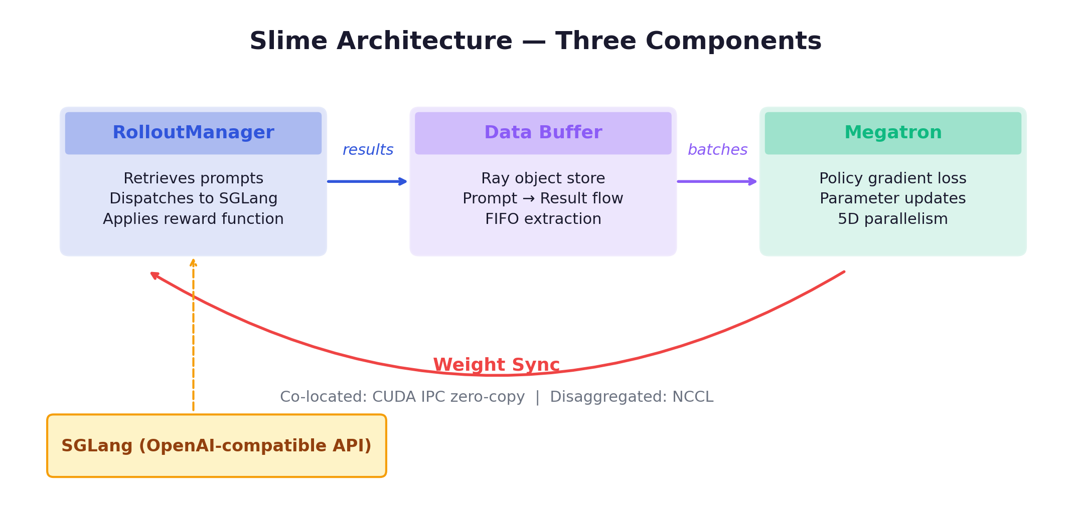
Three components:
Training Engine (Megatron-LM) with 5D parallelism (TP, PP, DP, CP, EP), dynamic batching, sequence packing, FP8 full-stack. As of v0.2.0, an alternative FSDP backend can directly load HuggingFace weights.
Rollout Engine (SGLang + sgl-router) provides a single HTTP endpoint with load balancing across SGLang instances. OpenAI-compatible API. StringRadixTrie for efficient prefix sharing (important for GRPO where G completions share the same prompt).
Data Buffer bridges training and rollout via Ray object store. Manages prompt initialization, custom data, and rollout generation results. Configurable extraction strategies (default: FIFO via pop_first).
The workflow:
Custom rollout logic is injected via --rollout-function-path — a standalone function with full access to SGLang’s async API, rather than framework subclassing:
       python -m slime.main \
    --rollout-function-path my_custom_rollout.py \
    --buffer-filter-path my_custom_filter.py
The custom function can implement arbitrary multi-turn, tool-calling, or tree-search patterns. This is far more flexible than the subclassing approach — and it means the framework’s core codebase doesn’t grow with each new use case.
Two Modes
Co-located (--colocate): training and inference share the same GPUs but run as separate processes. The system alternates between generation, training, and weight sync phases. Lower hardware barrier — works on a single 8-GPU node. But GPUs idle during the other phase, so there’s no parallelism between generation and training.
Decoupled (default): separate GPU clusters for rollout and training. Rollout engines continuously stream trajectories. No batch barriers. Continuous generation eliminates head-of-line blocking. This is what makes agentic RL with long-tail episodes practical — but it requires more total GPUs and an explicit weight sync mechanism.
APRIL Integration
For long-tail distributions, Slime integrates APRIL (Active Partial Rollouts): over-provision rollout requests, terminate once enough complete, recycle incomplete responses. Results: up to 44% rollout throughput improvement, up to 8% higher final accuracy.
Algorithms and Ecosystem
Supported: GRPO, DAPO, GSPO, PPO (v0.2.0+), REINFORCE++. Additional features: Multi-Token Prediction during RL, VLM support (Qwen3-VL), masked importance sampling.
Notable extensions: qqr (hilichurl) for open-ended agents using ArenaRL; Miles (RadixArk) with extra zero-copy weight sync optimizations; day-0 AMD ROCm support.
GLM-5’s Production Extensions to Slime
The GLM-5 technical report reveals several production-grade extensions to Slime that address real-world pain points at scale:
Multi-Task Rollout Orchestrator. GLM-5’s post-training spans diverse objectives — coding, terminal tasks, search agents, and on-policy distillation — each requiring different tool sets and rollout logic. Rather than building task-specific forks, each task registers its rollout and reward logic as an independent microservice. A central Multi-Task Rollout Orchestrator manages scheduling: it controls the per-task rollout ratio and generation speed, standardizes trajectories from all tasks into a unified message-list format, and supports 1k+ concurrent rollouts. This cleanly isolates task-specific logic from the core training loop.
Task advantage normalization. Architectural multi-task support (the Orchestrator above) is necessary but not sufficient — the algorithm must also handle the fact that different tasks produce advantages at very different scales. A coding task with 5% success rate produces sparse, high-magnitude advantages; a simpler web browsing task with 60% success rate produces dense, lower-magnitude advantages. Without correction, high-magnitude tasks dominate the gradient and other tasks stall. AgentRL (from the same THUDM / Z.AI team behind Slime) addresses this with per-task advantage normalization: for each task in a training batch, compute the mean and standard deviation of all token-level advantages across that task’s trajectories, then normalize: . This ensures every task contributes gradients with zero mean and unit variance, regardless of its intrinsic difficulty or reward density. Ablation studies show that removing this normalization causes training instability — the model learns different tasks at wildly different rates, with some tasks exhibiting reward fluctuations rather than steady improvement. The technique is complementary to GRPO’s group-relative normalization (which normalizes within a prompt group): GRPO handles intra-task variance, task advantage normalization handles inter-task variance.
Tail-latency optimization. For RL rollouts, the optimization target is not aggregate throughput but end-to-end latency — dominated by the slowest (long-tail) sample. GLM-5 addresses this on two fronts. First, Prefill-Decode (PD) disaggregation: in multi-turn settings, long-prefix prefills are frequent (conversation history, tool traces), and under DP-attention, a heavy prefill can preempt ongoing decodes on the same server. By running prefills and decodes on dedicated resources, decodes remain stable and uninterrupted — significantly improving tail behavior. Second, FP8 inference + Multi-Token Prediction (MTP): FP8 reduces per-token latency; MTP provides disproportionately large benefits on the long tail (rare long contexts, tool-heavy traces), reducing time-to-completion of the slowest sample and thus step-level stall time.
DP-aware routing for KV cache reuse. In multi-turn agentic workloads, sequential requests from the same rollout share an identical prefix. GLM-5 enforces rollout-level affinity: all requests belonging to a given agent instance are routed to the same DP rank via consistent hashing. This eliminates cross-rank cache misses, making prefill cost proportional to incremental tokens rather than total context length. Lightweight dynamic load rebalancing prevents long-term imbalance.
6. GPU-to-GPU Weight Transfer
This turned out to be one of the more technically interesting areas. The problem sounds simple — copy weights from training to inference — but the details make it genuinely hard.
The numbers involved: for a 70B model in bf16, that’s 140 GB of weights to transfer. For DeepSeek-V3 (671B MoE): over 1 TB. When a full training iteration takes 75-135 seconds, a weight transfer that takes minutes is a significant fraction of iteration time. And this happens every single step.
The Resharding Problem
The complexity isn’t just data transfer — it’s that training and inference use different parallelism layouts:
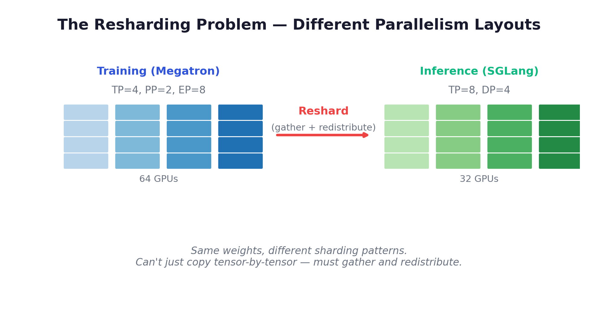
These are different sharding patterns of the same weights. You can’t just copy tensor-by-tensor. The weights must be gathered from the training topology and redistributed into the inference topology — a resharding operation that’s fundamentally a distributed systems coordination problem, not just a data movement problem. MoE models add another layer of complexity: expert parallelism means different experts may need different transfer topologies.
How Each Framework Handles It
Slime: CUDA IPC Zero-Copy
For co-located mode (Megatron and SGLang as separate processes on the same GPUs), Slime uses CUDA Inter-Process Communication — the most technically sophisticated approach I found for shared-GPU setups.
The process has five steps:
- Parameter Gathering: Megatron gathers distributed tensors from its parallelism layout (undoing TP/PP/EP sharding)
- CUDA IPC Handle Creation: Instead of copying the actual tensor data (GBs), tensors are serialized into CUDA IPC handles — lightweight pointers (~64 bytes each) to GPU memory locations
- Bucket Aggregation: Handles grouped into transfer-ready buckets to amortize IPC overhead
- Distribution: Handles sent to SGLang’s tensor parallel workers via
update_weights_from_tensor - Reconstruction: SGLang maps the handles and directly accesses tensor data in GPU memory — zero copy, zero serialization
The optimization journey is instructive:
| Stage | Time | What changed |
|---|---|---|
| Baseline | 60s | 81% spent on CUDA IPC open/close operations |
| + Tensor Flattening | ~25s | IPC ops reduced from 81% to 16% |
| + Bucketing | ~12s | Fewer individual transfers |
| + MoE-specific paths | 7s | Specialized handling for expert weights |
Result: Qwen3-30B-A3B in 7 seconds on 8×H100 — 8.5× speedup from baseline. The insight: the bottleneck wasn’t data transfer speed but the overhead of thousands of individual IPC open/close calls. Flattening tensors into contiguous buffers and bucketing them collapsed the IPC count dramatically.
For multi-node decoupled mode: UpdateWeightFromDistributed replaces CUDA IPC with NCCL.
VERL: 3D-HybridEngine Resharding
Training and generation use different 3D parallelism configurations on the same GPUs. FSDPVLLMShardingManager handles redistribution with zero memory redundancy — new parallel groupings formed by selecting ranks at regular intervals.
The v0.7 Checkpoint Engine adds bucket + pipeline support: 60%+ reduction in sync time. An experimental TransferQueue further decouples control flow from data flow with zero-copy and RDMA support.
Poolside: GPU-Direct NCCL
The fastest reported result: Llama 405B (810 GB in bf16) in ~2 seconds on P5e nodes with 8× H200 GPUs, 3200 Gbps EFAv3 networking, and GPUDirect RDMA. Fully asynchronous — training continues while weights transfer in the background.
The implementation supports different transfer patterns: simple 1-to-1 via NCCL point-to-point primitives, and N-to-M transfers via an abstract topology that defines what each GPU sends to each destination. Different tensors may need different routing (expert-parallel weights route differently from attention blocks).
What makes the Poolside write-up valuable is their candor about the engineering cost. At 10K GPUs, the challenges are qualitatively different from small-scale testing:
- Exact NCCL version matching required across all nodes — even slight mismatches cause silent bugs
- Frequent deadlocks from mismatched send/recv order in the N-to-M topology
- Resource contention across CUDA streams when training and transfer overlap
- Required warmup for all send/receive NCCL connections before production traffic
- Bugs that never appear on 8 GPUs surface immediately at 1000+
The recurring theme: small-scale stability doesn’t guarantee large-scale stability. This is probably the single most important lesson from their engineering blog for anyone building distributed RL systems.
TorchForge: TorchStore
A distributed in-memory KV store built on Monarch, optimized for PyTorch tensors with RDMA. Key design choice: lazy propagation (weights broadcast only when needed) and weight versioning for proper importance sampling correction in the replay buffer.
PrimeRL: File-Based Exchange
The simplest but slowest approach: trainer saves checkpoint to shared filesystem (NFS, S3), orchestrator detects new checkpoint, vLLM servers reload weights. Slow (minutes per sync), but it has one unique advantage: it works for cross-provider training where training runs on one cloud provider and inference on another. When there’s no shared GPU fabric, there’s no shared GPU memory — the filesystem becomes the only common substrate.
PrimeRL uses this for cross-datacenter RL, tolerating 2+ steps of staleness by necessity. The staleness is the price paid for provider flexibility.
MoonshotAI: Checkpoint-Engine Middleware
An engine-agnostic weight sync middleware used for Kimi-K2 training. The three-stage pipelined design — H2D (Host-to-Device) → Broadcast → Reload — allows each stage to proceed independently, overlapping computation where possible. The system falls back to serial mode when memory is too constrained for pipelining.
Updates 1-trillion-parameter models in ~20 seconds across thousands of GPUs. Specific measurement: 21.5s broadcast time for a 256×H20 setup.
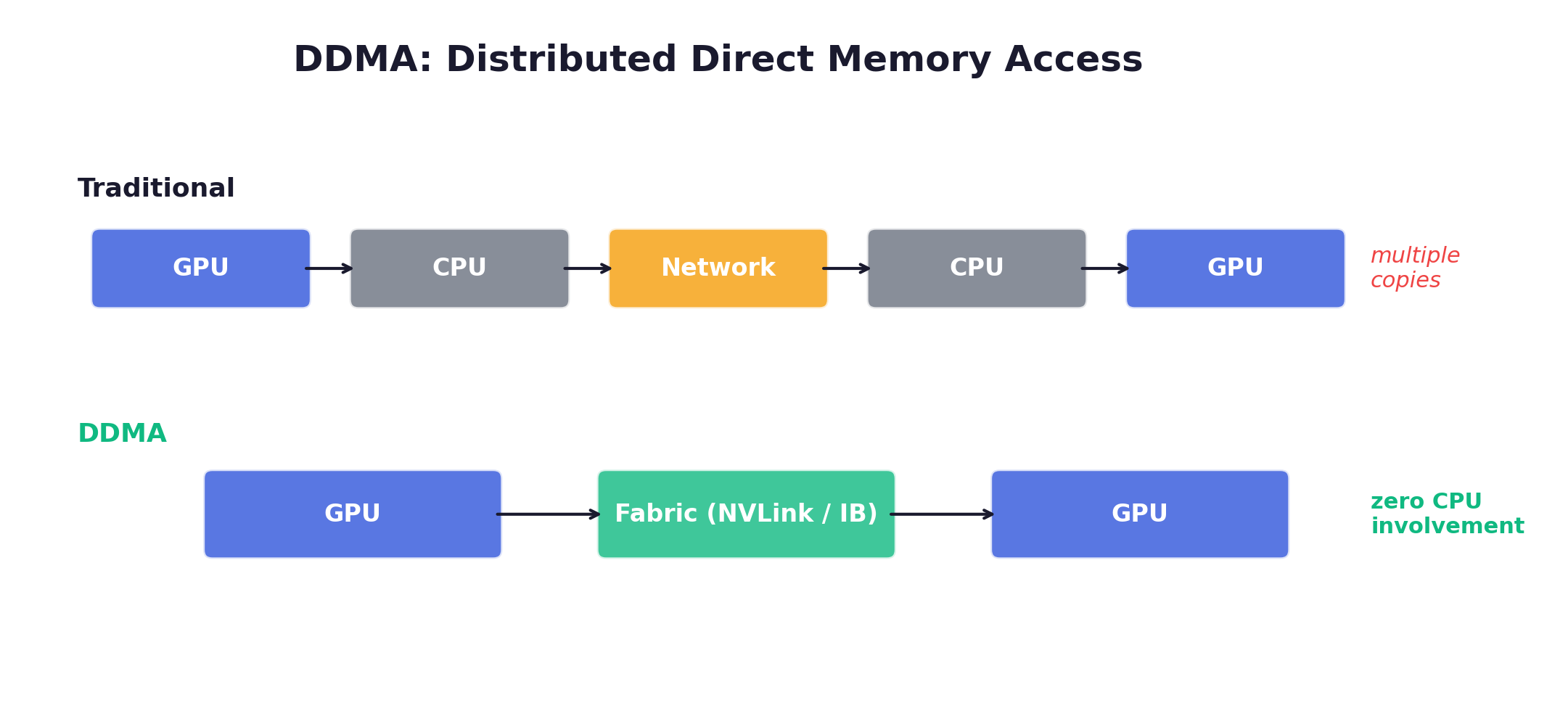
Future: DDMA
LlamaRL’s Distributed Direct Memory Access: GPU↔GPU over NVLink/InfiniBand with no host staging.
Comparison
| Mechanism | Speed | Async? | Multi-node? |
|---|---|---|---|
| Slime CUDA IPC | ~7s (30B) | No | Co-located only |
| VERL HybridEngine | ~10-15s (est.) | Yes (v0.7) | Yes |
| Poolside GPU-Direct | ~2s (405B) | Yes | Yes |
| TorchForge TorchStore | TBD | Yes | Yes |
| File-Based (PrimeRL) | Minutes | Yes | Yes |
| MoonshotAI Checkpoint | ~20s (1T) | Yes | Yes |
The co-located vs. disaggregated choice depends heavily on sync cost: if it’s fast (CUDA IPC at 7s), co-location is attractive; if it’s slow (file-based), disaggregation with overlap makes more sense.
7. Framework Comparison
The RL-for-LLMs framework ecosystem has exploded since DeepSeek-R1. Each framework embodies a distinct philosophy about how to structure the training system. Here’s what distinguishes them.
VERL (ByteDance)
Philosophy: Hybrid-Controller — single-controller flexibility with multi-controller efficiency.
The architecture is a two-level design: at the top level, a single RLTrainer process (the “single controller”) manages the global computation graph — it decides when to generate, when to train, and when to sync weights. But within each component, workers execute standard SPMD programs (the “multi controller” level) via FSDP/Megatron for training or vLLM/SGLang for inference. This hybrid approach gets the flexibility of centralized scheduling (one process can see the whole picture) with the performance of distributed execution (no centralized bottleneck during heavy computation).
Resource management: Ray placement groups allocate GPU resources. The max_colocate_count parameter controls how many roles share physical GPUs — critical for fitting PPO’s 4 models on limited hardware.
Key innovation: 3D-HybridEngine for in-place model resharding between training and generation phases. During training, the model might use TP=2, PP=1, DP=4 (optimized for gradient throughput). During generation, it reshards to TP=4, PP=1, DP=2 (optimized for inference latency). This happens on the same GPUs without duplicating the model — a significant memory savings.
Agentic support: VerlTool provides standardized tool APIs (code execution, search, SQL, vision). AgentLoopBase runs a per-conversation state machine, enabling trajectory-level async interaction without batch synchronization. Each conversation can be at a different turn, and completed trajectories are yielded to training immediately.
Scale: 1.53x to 20.57x throughput improvement over baselines (EuroSys 2025). Tested at 671B (DeepSeek-V3) on 96 H20 GPUs and Qwen3-235B on 32 H20 GPUs.
Algorithms: PPO, GRPO, GSPO, ReMax, REINFORCE++, RLOO, PRIME, DAPO, DrGRPO, KL_Cov, Clip_Cov, and more — the broadest algorithm coverage of any open-source framework. This breadth is one of VERL’s strongest selling points: if a new algorithm paper comes out, there’s a good chance someone in the community has already implemented it in VERL.
Slime (THUDM / Zhipu AI)
Philosophy: SGLang-native, inverted design where environments drive the framework. Covered in detail in Chapter 5.
Always maintains a server boundary — even in co-located mode. OpenAI-compatible API enables any environment to interact without modification.
Scale: Production system for GLM-4.5 (355B/32B MoE). 7s weight sync for 30B model.
TorchForge (Meta / PyTorch)
Philosophy: PyTorch-native, pseudocode-level expressiveness.
Built on Monarch (actor messaging framework) with a Services abstraction. The API is genuinely elegant:
       async def generate_episode(dataloader, policy, reference_model, reward, replay_buffer):
    prompt, target = await dataloader.sample.route()
    response = await policy.generate.route(prompt)
    ref_logprobs = await reference_model.forward.route(input_ids)
    reward_value = await reward.evaluate_response.route(prompt, response.text, target)
    await replay_buffer.add.route(Episode(...))
.route() for load-balanced routing, .fanout() for parallel broadcast. Integrates with torchtitan for training and vLLM for inference. Native OpenEnv integration (Gymnasium-style API, co-developed with Hugging Face).
Scale: 512 GPUs tested with Stanford and CoreWeave running GRPO. Still experimental — APIs may change, which is worth being aware of before building production systems on top of it. But for algorithm prototyping, the API clarity is hard to beat.
OpenRLHF
Philosophy: Ease of use first.
Distinct Ray actors for each role (Actor, Critic, Reward, Reference). One design decision worth noting: generation uses the vLLM engine with all its optimizations, while scoring (log-prob computation for the training loss) uses standard HuggingFace/DeepSpeed forward passes. The reasoning: generation benefits enormously from specialized inference optimizations (paged attention, continuous batching), but scoring is a simple forward pass that doesn’t need them. This pragmatic split avoids the complexity of making vLLM work for both use cases.
The most approachable framework for getting started — well-documented, mature community, straightforward configuration.
MiniMax Forge (Proprietary)
Philosophy: Agent-first, from the ground up.
The most distinctive feature: even black-box agents (binary executables) can be integrated via base URL redirect. The agent’s API endpoint is simply pointed at Forge’s inference engine during training. A Data Coordinator extracts sub-agent trajectories from execution logs. Forge requires implementing just four interfaces: agent_reprocess, agent_run, agent_postprocess, and calculate_reward — keeping the framework boundary minimal.
A notable insight from their M2.1 training: multi-scaffold training is essential for generalization. Different agent scaffolds introduce different context management and execution logic; training on a single scaffold (e.g., a simple ReAct loop) severely limits the model’s ability to generalize across deployment environments. This is an infrastructure requirement that’s easy to overlook — the framework must support running heterogeneous agent architectures within the same training loop.
Their CISPO algorithm (Clipped Importance Sampling Policy Optimization) is worth noting separately — it represents a genuinely different approach to the clip-ratio problem that’s been central to PPO and its successors.
The standard PPO clip operates on the surrogate objective: min(ratio * A, clip(ratio) * A). DAPO decouples the upper and lower clip bounds. CISPO takes a different path entirely: it clips the importance sampling weights themselves while preserving gradient updates for all tokens. The insight is that clipping the objective (as PPO does) can zero out gradients entirely for tokens with large importance ratios — wasting useful learning signal. CISPO clips the weights to control variance but keeps the gradient flowing.
Two practical lessons from scaling CISPO to agentic RL (M2.1): first, FP32 precision for the LLM head layer is critical — during M1 migration they discovered that reduced precision in the prediction layer caused significant training-inference inconsistency, and restoring FP32 resolved it (see Training-Inference Consistency for the full story). Second, multi-turn agent trajectories produce long-tail importance sampling ratios, so M2.1 added multiple importance sampling (MIS) and PPO-based trajectory filtering to discard trajectories with anomalous statistics before they destabilize training.
Result: 2× speedup over DAPO in controlled studies. Used to train MiniMax-M1 (512 H800 GPUs, 3 weeks) and subsequently M2.1 — a 230B-total / ~10B-activated MoE model.
[2026-02 Update] MiniMax M2.5 continued using CISPO and extended Forge with several notable improvements. First, a tree-structured merging strategy for training samples: in agentic RL, many trajectories share common prefixes (system prompt, initial observations, early reasoning steps). Forge now organizes these into a prefix tree, storing shared prefixes once and branching at divergence points — reportedly achieving ~40x training speedup by eliminating redundant computation. Second, a process reward mechanism for end-to-end monitoring of generation quality during agent execution, addressing the credit assignment challenge in long trajectories where a single outcome reward is insufficient. Third, the environment scale has grown dramatically: “most of the tasks and workspaces that we perform in our company have been made into training environments for RL — to date, there are already hundreds of thousands of such environments,” spanning R&D, product, sales, HR, and finance. M2.5 achieved 80.2% on SWE-bench Verified (surpassing Opus 4.6’s 78.9% on the Droid scaffold) while consuming fewer rounds (~20% fewer than M2.1) and running 37% faster per task.
Side-by-Side
| Dimension | VERL | Slime | TorchForge | OpenRLHF | MiniMax Forge |
|---|---|---|---|---|---|
| Training | FSDP / Megatron | Megatron / FSDP | torchtitan | DeepSpeed / Megatron | Internal |
| Inference | vLLM / SGLang | SGLang (native) | vLLM | vLLM | Internal + SGLang |
| Orchestration | Ray | Ray | Monarch | Ray | Internal |
| Weight Sync | In-process / Checkpoint Engine | CUDA IPC / Distributed | TorchStore (RDMA) | NCCL broadcast | Internal |
| Agentic RL | VerlTool + AgentLoop | Native (inverted design) | OpenEnv | Agent paradigm | Black-box agents |
| MoE Support | Full (EP, 5D) | Full (EP, FP8) | Via torchtitan | Varies | Internal |
| Maturity | Production (most mature OSS) | Production (GLM-4.x → GLM-5) | Experimental | Mature | Production (M1 → M2.5) |
| Key Metric | 20.57× throughput | 7s weight sync (30B) | 512 GPU tested | Ease of use | 2× speedup (CISPO), 40× tree merge |
The tradeoffs roughly map to: VERL for the broadest algorithm coverage and largest community; Slime for agentic RL with zero environment modification; TorchForge for staying in the PyTorch ecosystem with clean APIs; OpenRLHF for the fastest onboarding; and the MiniMax Forge pattern (base URL redirect) for integrating existing black-box agents — though implementing it requires building the machinery yourself since Forge is proprietary.
One thing that became clear during this survey: the “right” framework depends heavily on where in the async spectrum (Chapter 4) the workload falls. For simple math RLVR with synchronous training, any of these works and the choice is mostly about API ergonomics. For agentic RL with long-tail episodes, the architectural differences — Slime’s inverted design vs. VERL’s AgentLoop vs. TorchForge’s OpenEnv — become the dominant factor.
8. Scaling to Production — Patterns from Poolside
Poolside’s Model Factory is the most complete end-to-end RL training infrastructure publicly documented. Their blog series (6 parts) is worth reading in full. Here’s what stood out.
The Stack
10,000 H200 GPUs in a single Kubernetes cluster. AWS P5e nodes, 3200 Gbps EFAv3, GPUDirect RDMA.
| Layer | Technology | Purpose |
|---|---|---|
| Orchestration | Dagster | Workflow and asset management |
| Cluster | Kubernetes + Volcano scheduler | Batch scheduling, priority queues |
| Training | Titan (built on TorchTitan) | Pre-training, SFT, RL |
| Inference | Atlas (wraps vLLM) | Multi-platform: CUDA, ROCm, Trainium |
| Data | Apache Iceberg + Blender | Data lake with versioning + live streaming |
| Environments | Saucer + Task Engine | 800K+ repos, millions of concurrent executions |
| Metrics | Neptune + Grafana | Training metrics + monitoring |
| Incidents | incident.io | Automated alerting and escalation |
What Stood Out
Everything is a Dagster asset. Data tables, model checkpoints, experiment configs, evaluations — all versioned with full lineage. Any experiment can be reproduced exactly by referencing its asset versions. This also enables automated regression detection across training runs. Dagster is described as “the beating heart” of the Factory — it handles orchestration, scheduling, and dependency tracking across the entire pipeline.
Data is streamed, not materialized. Blender streams data into training — data mixes changeable live during training without stopping. This is especially important for online RL, where the data distribution shifts as the policy improves. Pre-materializing the training data would mean freezing the distribution, losing the ability to adapt the curriculum during training.
Evaluation is disaggregated. Evaluations scheduled independently from training, running every 100-1000 steps, across multiple benchmarks simultaneously. The signal from catching a regression at step 500 vs. discovering it at step 10,000 is enormous — it’s the difference between a 1-hour debugging session and a week-long investigation. Their philosophy: “No single evaluation is perfect — intelligence is multifaceted.”
Failure recovery is fully automated. At 10K GPUs, node failures are daily events. Their recovery pipeline:
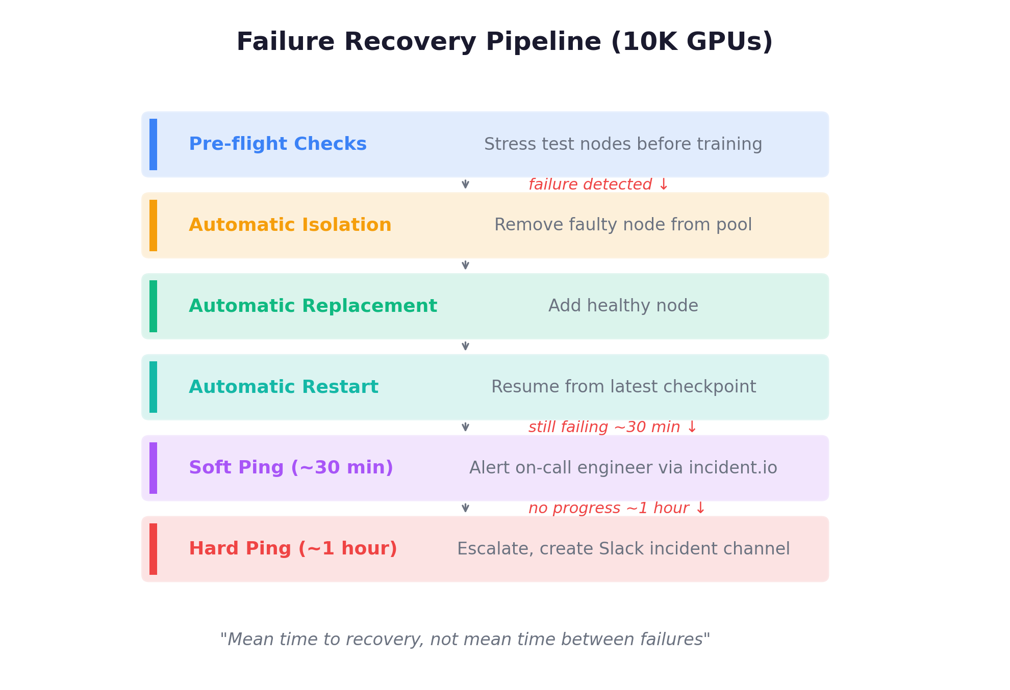
The metric that matters: mean time to recovery, not mean time between failures. At this scale, failures are assumed; recovery speed determines effective GPU utilization.
The self-improvement loop. Factory-trained agents help build container images for complex repositories (especially C++ projects that require understanding READMEs and debugging build systems). Better models → better infrastructure → better training data → better models. This is perhaps the most structurally interesting pattern: the system recursively improves itself, creating a flywheel that compounds over time.
Configuration as code. All experiments specified declaratively and version-controlled. Scheduling a new sweep takes <10 minutes with full reproducibility. Each parameter combination registered as a versioned Dagster asset. This sounds like table stakes, but in practice most research teams run experiments via ad-hoc config changes — making it impossible to answer “what exactly differed between run A and run B?” months later.
Profile before optimizing. Their first training framework (Monster) had excellent micro-benchmarks but was too rigid for rapid iteration. In their own telling, the lesson was that optimizing the wrong thing faster is still waste. They rebuilt with Titan (on TorchTitan) specifically to enable wider architectural changes at the cost of some micro-benchmark performance.
Heartbeat-driven fault tolerance (GLM-5). A complementary pattern from Slime’s production deployment: rollout servers periodically emit heartbeats monitored by the orchestration layer. Unhealthy servers are proactively terminated and deregistered from the inference router. Retries are automatically routed to healthy servers, preventing single-server incidents from interrupting rollouts and preserving uninterrupted end-to-end RL training. This is lighter-weight than Poolside’s full Dagster-based recovery pipeline, but addresses the same core insight: at scale, failures are assumed; automated recovery determines effective utilization.
9. Where Things Are Heading
A few trends that seem clear from this survey:
Server mode as default. Already the case in VERL v0.7, Slime, and TorchForge. Engine mode will persist for simple math RLVR on single nodes, but anything agentic requires server mode.
Standardized environment interfaces. OpenEnv (Meta + Hugging Face) is pushing a Gym-style step()/reset()/state() standard. Slime’s OpenAI-compatible API is complementary. Both reduce integration friction.
Training-serving convergence. Slime’s inverted design and VERL’s server mode both point toward a future where the inference engine used during RL training is the production serving engine. No separate deployment step.
GPU-direct transfers. DDMA and similar approaches will eliminate CPU bottlenecks in weight sync. As models grow, the transfer mechanism matters more.
Cross-provider training. PrimeRL already demonstrates cross-datacenter RL. As GPU availability fragments across providers, this becomes more common.
The gap between what’s possible with state-of-the-art infrastructure (Poolside’s ~2s weight sync, 10K GPU orchestration, self-improving agents) and what most research teams actually work with is enormous. The frameworks are closing that gap fast — VERL, Slime, and TorchForge each release major updates monthly. But the underlying principles seem stable:
Generation is the bottleneck. Async is essential for agentic RL. Weight sync speed determines iteration time. Decouple the components. Let environments drive the loop.
The infrastructure layer is increasingly where the real differentiation happens. Two teams running “GRPO on a 7B model” can get wildly different results depending on whether they’re using engine mode vs. server mode, sync vs. one-step-off-policy, and how they handle the long-tail distribution of agentic episodes. Understanding these differences is what this survey was about.
References
- Poolside Model Factory Blog Series (6 parts)
- Slime: SGLang-Native Post-Training Framework (LMSYS Blog)
- VERL: HybridFlow Paper (EuroSys 2025)
- TorchForge: PyTorch Blog
- Anatomy of RL Frameworks (Hanifleo)
- When LLMs Grow Hands and Feet: Agentic RL Systems (Amber Li)
- MiniMax-M1 Technical Report
- MiniMax M2.1: Post-Training Experience and Insights for Agent Models
- APRIL: Active Partial Rollouts in RL
- VerlTool: Agentic RL with Tool Use
- Open Source RL Libraries for LLMs (Anyscale)
- OpenEnv: Building the Open Agent Ecosystem (Hugging Face)
- GLM-4.5 Technical Report
- AReaL: Fully Asynchronous RL
- DAPO: Decoupled Clip and Dynamic Sampling
- DeepSeek-R1 Technical Report