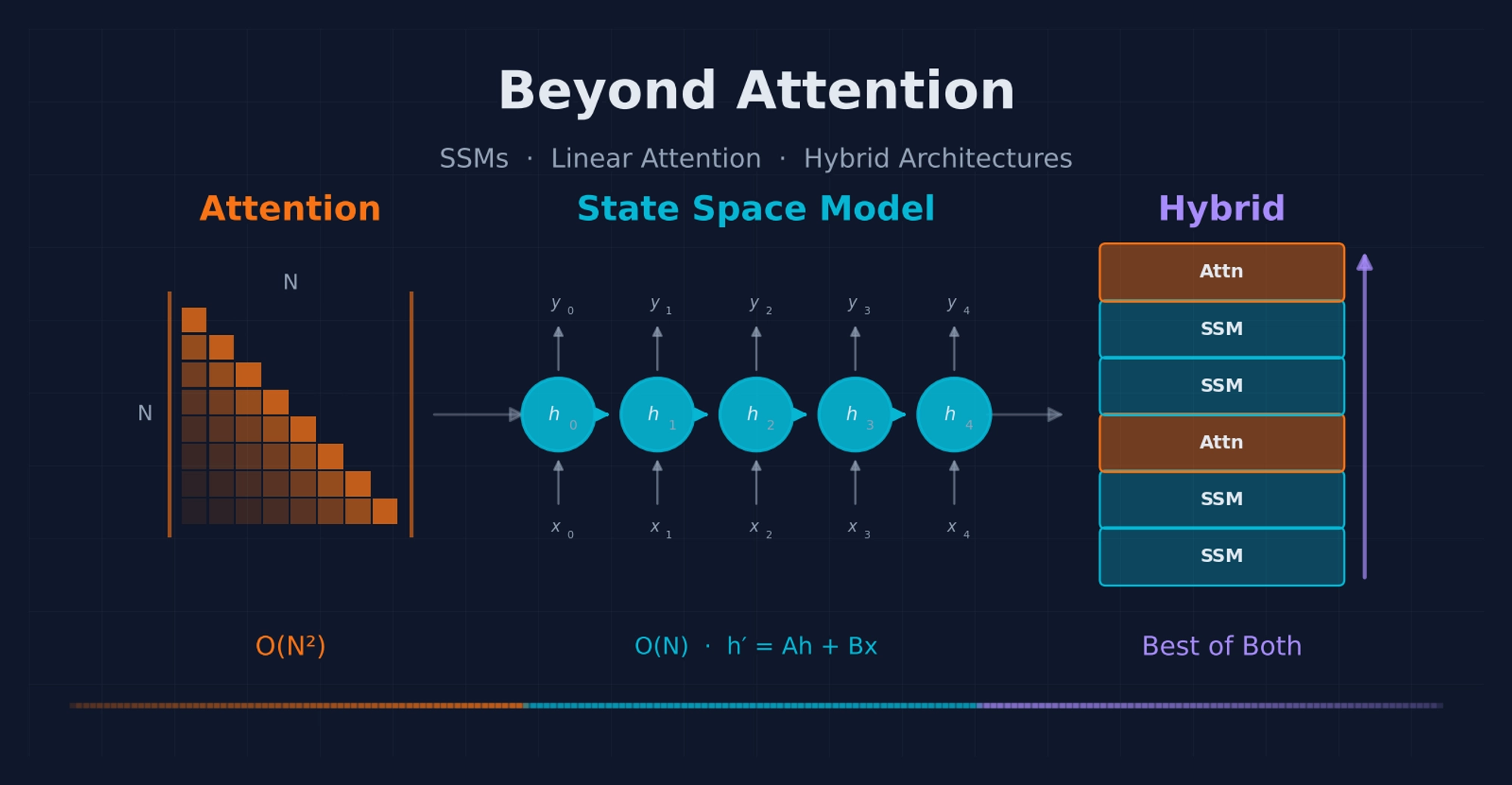
The future of sequence modeling isn’t attention OR recurrence — it’s knowing when to attend precisely and when to flow efficiently.
1. Why We Need Alternatives to Attention
The Transformer’s self-attention mechanism computes in both time and memory, where is the sequence length. For a 128K-token context window, the attention matrix contains 16.4 billion entries per layer per head. This quadratic scaling creates three concrete bottlenecks that are becoming increasingly painful in practice.
The Agentic RL Rollout Bottleneck
In reinforcement learning with verifiable rewards (RLVR), the training loop is: prompt → model generates rollout → environment verifies → reward signal → policy update. The generation (rollout) phase is autoregressive: each token depends on all previous tokens. With standard attention, this means:
| Step | Attend To | Operations |
|---|---|---|
| 1 | 1 token | 1 |
| 100 | 100 tokens | 100 |
| 10,000 | 10K tokens | 10,000 |
Even with KV caching, each new token requires attending to the entire cached history. For agentic tasks where the model interacts with tools, writes code, and iterates over multiple steps, rollouts easily reach 50K–100K tokens. The generation phase consumes 80-90% of total training time.
This is not a theoretical concern. Companies like Poolside have built elaborate async architectures specifically to hide this latency. But what if the model itself were simply faster at generation?
The Memory Wall
Modern reasoning tasks demand long contexts. The KV cache grows linearly: for each new token, we store a key and value vector for every layer and every head. At 128K tokens with a 7B parameter model in bf16, the KV cache alone exceeds the memory of most GPUs.
| Task Type | Context Length | KV Cache (7B, bf16) |
|---|---|---|
| Simple QA | 2K | ~256 MB |
| Code generation | 8K | ~1 GB |
| Multi-step agentic | 32K | ~4 GB |
| Repository-level coding | 128K | ~16 GB |
| Long-horizon planning | 256K+ | ~32 GB+ |
This creates a direct tension: we want models that can reason over long horizons, but attention makes long contexts prohibitively expensive.
Inference Cost at Scale
For production deployment, the economics are stark:
- Prefill (processing the prompt): — manageable with parallelism
- Decode (generating each new token): per token with KV cache
- Total decode cost for L output tokens:
When is large (long context) and is large (long generation), this becomes the dominant cost. A model that could maintain per-token generation — independent of context length — would fundamentally change the economics.
The Dream: Train Parallel, Infer Recurrent
The ideal architecture combines Transformer-like parallel training with RNN-like inference:
| Architecture | Training | Inference (per step) | State Size |
|---|---|---|---|
| Standard Attention | with KV cache | grows | |
| Linear Attention | fixed | ||
| S4 | fixed | ||
| Mamba | fixed | ||
| Mamba-2 | + tensor cores | fixed |
This turns out to be achievable. The key realization is that certain sequence models admit dual computation forms: one parallel (for training) and one recurrent (for inference), both computing the exact same function.
The Recall Problem
But there’s an elephant in the room worth addressing upfront: recall.
Standard attention can, in principle, attend to any token in the history with equal ease. This makes it excellent at tasks requiring precise retrieval — “What was the function name defined on line 47?” The attention matrix can place arbitrary weight on any position.
SSMs and linear attention variants compress the entire history into a fixed-size state. This compression is inherently lossy. The question is: how much recall capability do we sacrifice for efficiency, and can we get it back?
This tension — efficiency vs. recall — is the central design challenge of the field, and it’s what drives the evolution from pure SSMs to hybrid architectures that mix attention with SSM layers.
Roadmap
I spent a while working through the SSM and linear attention literature — papers, code, blog posts — trying to build a coherent picture of how these architectures relate to each other. This post is what came out of that process. It traces the evolution as I understand it:
- S4: The first SSM to match Transformers, via the convolution-recurrence duality
- Mamba: Making SSMs content-aware with selective parameters
- Mamba-2 (SSD): Revealing that SSMs and attention are two views of the same computation
- Linear Attention: The bridge connecting Transformers to RNNs through the associativity trick
- The Landscape: GLA, RWKV, RetNet, and the explosion of linear-time variants
- Hybrid Architectures: Jamba, Zamba, Samba — the pragmatic solution that combines attention and SSM layers
- Practical Implications: When to use what, and where the field is heading
Each section includes mathematical formulations, code implementations, and complexity analysis.
2. S4 — The Structured State Space Revolution
The SSM Foundation
A State Space Model describes a system that maintains an internal state x which evolves over time based on input u and produces output y:
Continuous-time SSM:
Where:
- is the hidden state ( = state dimension, typically 16-64)
- is the input signal
- is the state transition matrix
- maps input to state
- maps state to output
- is a skip connection (often set to 1)
To process discrete sequences (tokens), we need to discretize these continuous equations. S4 uses Zero-Order Hold (ZOH) with step size :
This gives us the discrete SSM:
In Python:
       def discretize_zoh(A, B, delta):
    """Zero-Order Hold discretization.
    A: (d_model, d_state) — diagonal state transition
    B: (d_model, d_state) — input-to-state mapping
    delta: (d_model,)     — step size per dimension
    """
    A_bar = torch.exp(delta.unsqueeze(-1) * A)  # exp(Δ·A)
    B_bar = delta.unsqueeze(-1) * B              # Δ·B (first-order)
    return A_bar, B_bar
An alternative discretization method is the bilinear transform (Tustin’s method), which is more accurate but slightly more expensive:
       def discretize_bilinear(A, B, delta):
    """Bilinear (Tustin) discretization — more accurate for oscillatory systems"""
    dA = delta.unsqueeze(-1) * A * 0.5
    A_bar = (1 + dA) / (1 - dA)    # (1 + Δ/2·A) / (1 - Δ/2·A)
    B_bar = delta.unsqueeze(-1) * B / (1 - dA)
    return A_bar, B_bar
ZOH is simpler and works well for monotonic decay dynamics; bilinear preserves frequency content better. S4 uses ZOH; some follow-up works use bilinear.
The Dual Forms: S4’s Key Insight
The key insight is that the discrete SSM can be computed in two mathematically equivalent ways.
Form 1: Recurrence — per step, perfect for inference
Process tokens one at a time, maintaining state:
       def ssm_recurrent(u, A_bar, B_bar, C, D):
    """O(N) total, O(1) per step — perfect for autoregressive generation"""
    batch, L, d_model = u.shape
    x = torch.zeros(batch, d_model, d_state)  # fixed-size state

    outputs = []
    for t in range(L):
        x = A_bar * x + B_bar * u[:, t, :].unsqueeze(-1)
        y_t = (C * x).sum(dim=-1) + D * u[:, t, :]
        outputs.append(y_t)

return torch.stack(outputs, dim=1)Pros: Constant memory, per token — no matter how long the context Cons: Sequential — can’t parallelize across time steps, so training is slow
Form 2: Convolution — parallel, perfect for training
Unrolling the recurrence reveals a convolution. Consider the first few outputs:
The pattern reveals a convolution with kernel :
Then: (1D convolution), computable via FFT in .
       def compute_ssm_kernel(A_bar, B_bar, C, L):
    """Compute convolution kernel K[t] = C · A_bar^t · B_bar

    The kernel only depends on A, B, C, Δ — NOT on the input.
    Precompute once for a given sequence length and reuse for all sequences.
    """
    powers = torch.arange(L, device=A_bar.device).float()
    A_powers = A_bar.unsqueeze(-1) ** powers    # (d_model, d_state, L)
    kernel = torch.einsum('dn,dn,dnl->dl', C, B_bar, A_powers)
    return kernel  # (d_model, L)

def ssm_conv_mode(u, K, D):
    """O(N log N) via FFT — perfect for training"""
    u_t = u.transpose(1, 2)         # (batch, d_model, L)
    n_fft = 2 * u.shape[1]          # pad to avoid circular convolution

    u_fft = torch.fft.rfft(u_t, n=n_fft, dim=-1)
    K_fft = torch.fft.rfft(K, n=n_fft, dim=-1)
    y_fft = u_fft * K_fft.unsqueeze(0)
    y = torch.fft.irfft(y_fft, n=n_fft, dim=-1)[..., :u.shape[1]]

return y.transpose(1, 2) + D * uPros: Fully parallel, exploits FFT hardware Cons: memory for the kernel, time
Why Both Forms Compute the Same Thing
This equivalence holds because the SSM is a Linear Time-Invariant (LTI) system. For any LTI system:
- The impulse response (kernel K) completely characterizes the input-output relationship
- The output is the convolution of input with the impulse response
- But you can also compute this incrementally via the recurrence
The kernel only depends on A, B, C, and Δ — not on the input. So you can precompute it once for a given sequence length and reuse it for all sequences. During training, you use the convolution form (parallel). During inference, you switch to recurrence form ( per step). The model computes the exact same function either way.
This dual computation pattern — parallel for training, recurrent for inference — is the central principle that all subsequent SSM and linear attention architectures exploit.
HiPPO: Why Initialization Matters
S4’s other key contribution is the HiPPO (High-order Polynomial Projection Operator) framework for initializing the A matrix.
Random initialization of A leads to either:
- Rapid decay: information is forgotten too quickly (eigenvalues too negative)
- Instability: states explode (eigenvalues with positive real parts)
HiPPO provides a principled initialization based on optimally compressing the history using orthogonal polynomials (specifically, Legendre polynomials). The idea: at each timestep, the state should be the best polynomial approximation of the entire input history seen so far.
The diagonal approximation:
       def make_hippo_diagonal(N):
    """A_n = -(n + 1/2) for n = 0, 1, ..., N-1
    Each dimension decays at a different rate, creating multi-scale memory:
      - Dimension 0:  decay 0.5  (slow, captures long-range patterns)
      - Dimension 15: decay 15.5 (medium, captures mid-range context)
      - Dimension 63: decay 63.5 (fast, captures fine local detail)
    """
    return -(torch.arange(N).float() + 0.5)
This multi-scale memory is what allows S4 to handle sequences of 16,000+ tokens — far beyond what LSTMs and GRUs could achieve. The slow dimensions remember events from thousands of steps ago; the fast dimensions capture recent local patterns. Together, they form a multi-resolution representation of the entire history.
S4: Putting It All Together
The complete S4 layer combines discretization, dual-mode computation, and HiPPO initialization:
       class S4Layer(nn.Module):
    def __init__(self, d_model, d_state=64):
        super().__init__()
        # SSM parameters (diagonal form for efficiency)
        self.A_log = nn.Parameter(
            torch.log(make_hippo_diagonal(d_state).abs() + 1e-4)
            .unsqueeze(0).expand(d_model, -1).clone()
        )
        self.B = nn.Parameter(torch.randn(d_model, d_state) * 0.1)
        self.C = nn.Parameter(torch.randn(d_model, d_state) * 0.1)
        self.D = nn.Parameter(torch.ones(d_model))
        self.log_delta = nn.Parameter(
            torch.log(torch.ones(d_model) * 0.01)  # Small initial step size
        )
        self._kernel_cache = None
        self._cached_length = 0

    def forward(self, u, state=None):
        """Training: convolution form. Inference: recurrence form."""
        A = -torch.exp(self.A_log)
        delta = torch.exp(self.log_delta)
        A_bar, B_bar = discretize_zoh(A, self.B, delta)

        if state is not None:
            # Inference mode: O(1) per step recurrence
            return ssm_recurrent(u, A_bar, B_bar, self.C, self.D, state)
        else:
            # Training mode: O(N log N) convolution
            L = u.shape[1]
            K = compute_ssm_kernel(A_bar, B_bar, self.C, L)
            return ssm_conv_mode(u, K, self.D)

    def step(self, u_t, state):
        """O(1) single step for autoregressive generation.
        u_t: (batch, d_model) — single token
        state: (batch, d_model, d_state) — running SSM state
        """
        A = -torch.exp(self.A_log)
        delta = torch.exp(self.log_delta)
        A_bar, B_bar = discretize_zoh(A, self.B, delta)

        state = A_bar * state + B_bar * u_t.unsqueeze(-1)
        y_t = (self.C * state).sum(dim=-1) + self.D * u_t
        return y_t, state
Note the step() method: during autoregressive generation, we call this once per token. The state is a fixed-size tensor of shape (batch, d_model, d_state) — typically around 64 floats per dimension. No matter how many tokens we’ve generated, the state never grows.
S4’s Limitation: Time-Invariance
S4 has one fundamental weakness: A, B, C, and Δ are fixed parameters — they don’t depend on the input. This means:
- Every token is processed with the same transition dynamics
- The model can’t selectively remember or forget based on content
- It’s like reading a book where you highlight every word with the same color
Consider: “The capital of France is ___. France is in Europe.”
An S4 model processes both “France” tokens identically. It can’t decide that the first “France” (in a question context) should be strongly encoded while the second (in a statement context) is less important. The kernel K is precomputed and applies uniformly to all inputs.
This is the fundamental tradeoff of LTI systems: the convolution trick that enables training requires time-invariance. Making parameters input-dependent breaks the convolution — which means we need a new parallel computation strategy.
S4 Complexity Summary
| Aspect | S4 | Standard Attention |
|---|---|---|
| Training | via FFT | |
| Inference per step | with KV cache | |
| State size | ≈ 64 floats | grows with context |
| Long sequences | Excellent (via HiPPO) | Quadratic cost |
| Content awareness | None (time-invariant) | Full (softmax attention) |
| Kernel precompute | Yes — reuse across sequences | N/A |
3. Mamba — Making SSMs Content-Aware
The Selection Mechanism
Mamba’s core innovation is making SSM parameters input-dependent:
S4 (Time-Invariant) — same for all timesteps:
Mamba (Selective) — parameters depend on current input:
The parameters serve distinct roles:
- B_t (input-dependent): Controls what information to write to the state — “what should we remember about this token?”
- C_t (input-dependent): Controls what information to read from the state — “what past context is relevant right now?”
- Δ_t (input-dependent): Controls the importance of the current token — high Δ means “this token matters, encode it strongly”; low Δ means “pass through, don’t disrupt the state”
- A (fixed, NOT input-dependent): Controls the base decay rate — how quickly old information fades
Note that A is deliberately NOT input-dependent. This is a design choice: A controls the fundamental decay dynamics of the state, which can be learned but don’t need to vary per-token. Making A input-dependent would increase the parameter count and computation without significant quality gains. B and C control the read/write operations, which do need input-dependent flexibility. Δ controls how much the current timestep “matters,” effectively modulating how strongly A’s decay is applied.
Why Selection Matters: The Copy Task Intuition
Consider: “The capital of France is ___. France is in Europe.”
S4 (time-invariant): Every token gets the same write strength to the state. Both “France” tokens are processed identically. “The” and “is” receive the same encoding effort as “capital” and “France.” The model can’t decide which tokens are important — it’s like a camera with a fixed exposure.
Mamba (selective): The model can:
- Strongly write the “France” → “capital” association (high Δ, informative B) — this token matters
- Weakly write filler tokens like “is” and “in” (low Δ) — these are structural, not semantic
- Selectively forget irrelevant context (via A decay modulated by Δ) — clear space for new important information
This is like a camera with adaptive exposure: bright for important subjects, dark for the background.
The copy task makes this even clearer: given “ABCDE…copy…ABCDE”, the model must remember the initial sequence and reproduce it. S4 treats the “copy” token the same as “A” — it can’t signal “now start reading from state.” Mamba can make Δ very small during the “copy” token (don’t write, just pass through) and then use C to read the relevant stored information.
The Challenge: No More Convolution
With input-dependent parameters, S4’s convolution trick breaks completely. The kernel was precomputable because were the same for all inputs. In Mamba, , , and differ for every token — there’s no single kernel to precompute.
Naive approaches:
- Process sequentially: but no parallelism → slow training on GPUs
- Materialize the full matrix: → defeats the purpose of using an SSM
The Parallel Scan Solution
Mamba’s answer is the parallel scan (also called prefix sum) algorithm. The key insight is that the SSM recurrence is associative:
Given two consecutive operations and , where each computes , their composition is:
This works because: if x₁ = A₁·x₀ + b₁ and x₂ = A₂·x₁ + b₂, then x₂ = A₁·A₂·x₀ + A₂·b₁ + b₂. The combined operation is still a linear function of x₀, with the same (multiply, add) structure.
Because this operation is associative (but not commutative), we can use parallel prefix computation:
- Total work: — same as sequential
- Parallel depth: — with processors, we finish in steps
- In practice: Implemented as a custom CUDA kernel with careful memory management
       # Conceptual parallel scan (actual Mamba uses fused CUDA kernels)
def parallel_scan_associative(A_bars, B_bar_u):
    """
    A_bars:  (batch, L, d_inner, d_state) — per-step decay
    B_bar_u: (batch, L, d_inner, d_state) — per-step input contribution

    Returns: all hidden states x_1, x_2, ..., x_L

    The algorithm works in O(log L) parallel rounds:
    Round 1: combine pairs (1,2), (3,4), (5,6), ...
    Round 2: combine results at distance 2, 4, 8, ...
    After log(L) rounds, all prefix sums are computed.
    """
    # This is O(N) total work, O(log N) depth
    # Real implementation uses mamba_ssm.ops.selective_scan_cuda
    pass
The Selective Scan: Step by Step
Here’s the complete selective scan in explicit sequential form (the parallel scan computes the same result):
       def selective_scan(u, delta, A, B, C, D):
    """Core Mamba operation — sequential reference implementation.

    u:     (batch, L, d_inner) — expanded input
    delta: (batch, L, d_inner) — input-dependent step size
    A:     (d_inner, d_state)  — FIXED state transition (negative values)
    B:     (batch, L, d_state) — input-dependent write gate
    C:     (batch, L, d_state) — input-dependent read gate
    D:     (d_inner,)          — skip connection

    Returns: (batch, L, d_inner) — output sequence
    """
    batch, L, d_inner = u.shape
    d_state = A.shape[1]
    x = torch.zeros(batch, d_inner, d_state)  # Hidden state

    outputs = []
    for t in range(L):
        # Step 1: Discretize with input-dependent delta
        #   Large delta → strong update (token matters)
        #   Small delta → weak update (token is filler)
        delta_A = delta[:, t, :].unsqueeze(-1) * A     # (batch, d_inner, d_state)
        A_bar_t = torch.exp(delta_A)                     # Decay factor

        # Step 2: Input contribution = delta * B * u
        #   This is the "write" operation: encoding the current token
        delta_B_u = (delta[:, t, :].unsqueeze(-1)         # importance
                     * B[:, t, :].unsqueeze(1)             # write gate
                     * u[:, t, :].unsqueeze(-1))           # content

        # Step 3: State update — decay old state, add new input
        x = A_bar_t * x + delta_B_u

        # Step 4: Output — read from state + skip connection
        y_t = (x * C[:, t, :].unsqueeze(1)).sum(dim=-1) + D * u[:, t, :]
        outputs.append(y_t)

    return torch.stack(outputs, dim=1)
The Full Mamba Block
Mamba wraps the selective SSM in a gated architecture inspired by Gated Linear Units:
       class MambaBlock(nn.Module):
    def __init__(self, d_model, d_state=16, d_conv=4, expand=2):
        super().__init__()
        d_inner = d_model * expand

        # 1. Input projection → x (main path) and z (gating branch)
        self.in_proj = nn.Linear(d_model, d_inner * 2, bias=False)

        # 2. Depthwise convolution for local context
        self.conv1d = nn.Conv1d(d_inner, d_inner, kernel_size=d_conv,
                                padding=d_conv-1, groups=d_inner)

        # 3. Selective parameter projections
        self.x_proj = nn.Linear(d_inner, d_state * 2, bias=False)  # B, C
        self.dt_proj = nn.Linear(d_inner, d_inner, bias=True)       # delta

        # 4. Fixed A (not input-dependent) — initialized as log-spaced decay
        self.A_log = nn.Parameter(torch.log(
            torch.arange(1, d_state + 1).float()
        ).unsqueeze(0).expand(d_inner, -1).clone())
        self.D = nn.Parameter(torch.ones(d_inner))

        # 5. Output projection
        self.out_proj = nn.Linear(d_inner, d_model, bias=False)

    def forward(self, x):
        # Split into main path and gating path
        xz = self.in_proj(x)                            # (batch, L, 2*d_inner)
        x_inner, z = xz.chunk(2, dim=-1)

        # Local context via depthwise conv1d
        x_conv = self.conv1d(x_inner.transpose(1, 2))[:, :, :x.shape[1]]
        x_conv = F.silu(x_conv.transpose(1, 2))

        # Generate selective parameters from conv-processed input
        BC = self.x_proj(x_conv)
        B, C = BC.chunk(2, dim=-1)
        delta = F.softplus(self.dt_proj(x_conv))
        A = -torch.exp(self.A_log)

        # Selective scan — the core SSM computation
        y = selective_scan(x_conv, delta, A, B, C, self.D)

        # Gating: y_final = y * SiLU(z)
        y = y * F.silu(z)
        return self.out_proj(y)
Why Conv1d Before the SSM?
The depthwise convolution (kernel size typically 4) serves multiple purposes:
- Local context window: Provides n-gram-like local information that the SSM can use when computing its selective parameters. Without it, B_t and C_t would depend only on the current token embedding, missing crucial local context.
- Compensates for smoothing: SSMs tend to smooth over local patterns due to their recurrent nature. The conv captures sharp local features.
- Computationally cheap:
groups=d_innermeans each channel is convolved independently — no cross-channel interaction, so the cost is . - Analogous to positional cues: Provides local structure similar to how positional encodings work in Transformers.
The Gating Mechanism
The z branch is a separate projection of the input that acts as a learned gate, similar to the Gated Linear Unit (GLU) family (SwiGLU, GEGLU, etc.). This:
- Helps gradient flow through the network (z provides a direct path)
- Provides feature selection independent of the SSM dynamics — some features may be passed through directly
- Is standard in modern architectures and empirically beneficial
O(1) Inference: The Step Function
For autoregressive generation, we only need to process one token at a time. This is where Mamba’s fixed-state advantage shines:
       def step(self, x_t, conv_state, ssm_state):
    """O(1) per token — the whole point of using SSMs.

    x_t:        (batch, d_model)             — single token embedding
    conv_state: (batch, d_inner, d_conv-1)   — sliding window for conv
    ssm_state:  (batch, d_inner, d_state)    — SSM hidden state

    Returns: y_t, new_conv_state, new_ssm_state
    """
    # Input projection
    xz = self.in_proj(x_t)                   # (batch, 2*d_inner)
    x_inner, z = xz.chunk(2, dim=-1)

    # Conv: shift the sliding window and apply convolution
    conv_full = torch.cat([conv_state, x_inner.unsqueeze(-1)], dim=-1)
    x_conv = (conv_full * self.conv1d.weight.squeeze(1)).sum(dim=-1)
    x_conv = x_conv + self.conv1d.bias
    x_conv = F.silu(x_conv)
    conv_state = conv_full[:, :, 1:]         # Slide window forward

    # Generate selective parameters for this single token
    BC = self.x_proj(x_conv)
    B, C = BC.chunk(2, dim=-1)
    delta = F.softplus(self.dt_proj(x_conv))
    A = -torch.exp(self.A_log)

    # Single SSM step: O(d_inner × d_state) ≈ O(d²)
    A_bar = torch.exp(delta.unsqueeze(-1) * A)
    delta_B_u = delta.unsqueeze(-1) * B.unsqueeze(1) * x_conv.unsqueeze(-1)
    ssm_state = A_bar * ssm_state + delta_B_u
    y = (ssm_state * C.unsqueeze(1)).sum(dim=-1) + self.D * x_conv

    # Gating and output
    y = y * F.silu(z)
    return self.out_proj(y), conv_state, ssm_state
The total state per layer consists of:
- conv_state:
(d_inner, d_conv-1)— sliding window for the convolution, typically(128, 3)≈ 384 floats - ssm_state:
(d_inner, d_state)— the SSM hidden state, typically(128, 16)≈ 2,048 floats
Compare to a Transformer’s KV cache per layer at 100K context:
- KV cache:
(2 × n_heads × head_dim × 100K)≈ 100M+ values
That’s roughly a 50,000x reduction in per-layer state. This is why Mamba can generate tokens at long contexts without the memory bottleneck that plagues Transformers.
What Mamba Achieves
| Aspect | Transformer | Mamba |
|---|---|---|
| Training | via parallel scan | |
| Inference per step | — independent of | |
| KV cache / state | — grows linearly | — constant |
| Long context | Expensive | Near-free |
| Content awareness | Full (softmax) | Selective (input-dependent B, C, Δ) |
| Hardware | Standard matmul → tensor cores | Custom CUDA kernels |
The Falcon Mamba 7B model, trained on 5.8 trillion tokens, surpassed Mistral 7B, Llama 3.1 8B, and Falcon2 11B on the Open LLM Leaderboard — a strong signal that pure SSM architectures can compete at scale.
The Remaining Question
Mamba’s parallel scan relies on custom CUDA kernels hand-tuned for GPU memory hierarchies. This works, but:
- It’s hard to maintain and port across hardware
- It can’t leverage tensor cores — the fastest hardware path on modern GPUs (optimized for matrix multiplication, not scan)
- Custom kernels are a bottleneck for adoption
What if we could express the SSM computation as standard matrix multiplication, letting us use the most optimized hardware path available?
That’s exactly what Mamba-2 achieves.
4. Mamba-2: The State Space Duality Revealed
SSM = Semi-Separable Matrix Multiplication
Mamba-2’s breakthrough is revealing a deep mathematical connection: SSM computation is equivalent to multiplication by a semi-separable matrix. This connects SSMs to attention at a fundamental level and enables using tensor cores.
Consider the SSM output unrolled:
This can be written as a matrix multiplication , where:
This matrix is semi-separable: each element is a product of three factors — a row factor (), a decay factor (), and a column factor (). It’s lower-triangular (causal) with exponential decay away from the diagonal.
We can build it explicitly:
       def build_semiseparable_matrix(A, B, C, L):
    """Build the semi-separable matrix M[i,j] = C_i · diag(A^{i-j}) · B_j

    This makes the SSM-attention duality concrete:
    - Standard attention: M = softmax(Q @ K^T / √d)
    - SSD (SSM):         M[i,j] = C_i · A^{i-j} · B_j

    A: (d_state,) — decay values (scalar per state dimension)
    B: (L, d_state) — per-position "key" (write gate)
    C: (L, d_state) — per-position "query" (read gate)
    """
    positions = torch.arange(L)
    diff = positions.unsqueeze(0) - positions.unsqueeze(1)  # (L, L)

    # Decay matrix: A^{i-j} for each state dimension
    D = A.view(-1, 1, 1) ** diff.clamp(min=0).unsqueeze(0)  # (d_state, L, L)

    # Apply causal mask
    causal_mask = torch.tril(torch.ones(L, L))
    D = D * causal_mask.unsqueeze(0)

    # M[i,j] = Σ_k C[i,k] · D[k,i,j] · B[j,k]
    M = torch.einsum('id,dij,jd->ij', C, D, B)
    return M  # (L, L) — the full semi-separable matrix
The SSM-Attention Connection
Now compare with standard attention:
| Standard Attention | SSD (Mamba-2) | |
|---|---|---|
| Matrix | ||
| Query/Key | (read gate), (write gate) | |
| Value | (input) | |
| Pattern | Softmax → sharp, content-dependent | Exponential decay → smooth, distance-dependent |
| Normalization | Softmax (sum-to-1) | None (implicit via decay) |
| Complexity | to materialize | via recurrence |
Both are bilinear in query and key: the output at position depends on the interaction between what we want to read ( / ) and what was written ( / ). The critical difference:
- Attention uses softmax normalization → creates sharp attention patterns that can focus on specific tokens regardless of distance
- SSD uses exponential decay → creates smooth patterns where recent tokens are weighted more heavily
This is the Structured State Space Duality (SSD): SSMs and attention are two ends of a spectrum, connected by the semi-separable matrix structure. One uses content-based routing (softmax), the other uses position-based decay (exponential). Both compute where is structured differently.
Chunked Computation: Tensor Cores Meet RNNs
The matrix has size — materializing it fully would be , defeating the purpose. Mamba-2’s key optimization is chunked processing:
- Divide the sequence into chunks of size (e.g., )
- Within each chunk: Use the matrix form — a small matmul → tensor cores!
- Between chunks: Pass state via recurrence — like an RNN
       def ssm_chunked(x, A, B, C, chunk_size=64):
    """Chunked SSD computation.

    Within chunk: matrix form (tensor core acceleration)
    Between chunks: state passing (O(1) per chunk boundary)
    Total: O(N/P · P²) = O(N·P) — for fixed P, this is O(N)

    The small P×P matrices fit in registers/shared memory,
    and matrix multiplication is the most optimized operation
    on H100/H200 GPUs via tensor cores.
    """
    batch, L, d_inner = x.shape
    d_state = A.shape[-1]
    state = torch.zeros(batch, d_inner, d_state)

    all_outputs = []
    for start in range(0, L, chunk_size):
        end = min(start + chunk_size, L)
        P = end - start

        x_chunk = x[:, start:end, :]        # (batch, P, d_inner)
        B_chunk = B[:, start:end, :]         # (batch, P, d_state)
        C_chunk = C[:, start:end, :]         # (batch, P, d_state)

        # BUILD the P×P semi-separable matrix for this chunk
        # M_chunk[i,j] = C_chunk[i] @ diag(A^{i-j}) @ B_chunk[j]
        # This is a small matmul → tensor cores handle it efficiently

        # APPLY: y_chunk = M_chunk @ x_chunk
        # PLUS: contribution from inter-chunk state

        # UPDATE state for next chunk
        # state encodes the effect of all tokens before this chunk

        chunk_outputs = []
        for t in range(P):
            state = A * state + B_chunk[:, t, :].unsqueeze(1) * x_chunk[:, t, :].unsqueeze(-1)
            y_t = (C_chunk[:, t, :].unsqueeze(1) * state).sum(dim=-1)
            chunk_outputs.append(y_t)

        all_outputs.append(torch.stack(chunk_outputs, dim=1))

    return torch.cat(all_outputs, dim=1), state
Why This Is a Breakthrough
Mamba-1 (parallel scan):
- Custom CUDA kernels hand-tuned for each GPU architecture
- Can’t leverage tensor cores (the fastest operation on modern GPUs)
- Hard to maintain, debug, and port
- Each hardware generation needs new kernel tuning
Mamba-2 (chunked SSD):
- Standard matrix multiplication within chunks → tensor cores
- Uses existing highly-tuned BLAS libraries (cuBLAS, etc.)
- More portable across hardware (tensor cores are universal)
- Easier to understand, maintain, and optimize
- Enables Triton implementations (more accessible than raw CUDA)
The practical speedup: 2-8x higher throughput over Mamba-1 on the same hardware.
The Multi-Head SSD Layer
Like attention, Mamba-2 uses multiple heads, each with its own SSD computation:
       class SSD(nn.Module):
    """Multi-head Structured State Space Duality layer.

    Analogous to multi-head attention:
    - Input → project to B (key), C (query), x (value)
    - Each head: independent SSD computation
    - Concatenate heads → output projection
    """
    def __init__(self, d_model, n_heads=8, d_state=64, chunk_size=64):
        super().__init__()
        self.head_dim = d_model // n_heads
        self.n_heads = n_heads
        self.d_state = d_state
        self.chunk_size = chunk_size

        # Projections (analogous to Q, K, V in attention)
        self.in_proj = nn.Linear(d_model, d_model * 3, bias=False)

        # Decay parameter per head — learned
        self.A_log = nn.Parameter(torch.randn(n_heads, self.head_dim))

        self.out_proj = nn.Linear(d_model, d_model, bias=False)

    def forward(self, x):
        batch, L, _ = x.shape

        # Project: x → (B-like, C-like, input)
        x_inner, B_proj, C_proj = self.in_proj(x).chunk(3, dim=-1)

        # Reshape for multi-head: (batch, L, n_heads, head_dim)
        x_inner = x_inner.view(batch, L, self.n_heads, self.head_dim)
        B_proj = B_proj.view(batch, L, self.n_heads, self.head_dim)
        C_proj = C_proj.view(batch, L, self.n_heads, self.head_dim)

        # Decay in (0, 1) for stability
        A = torch.sigmoid(self.A_log)  # (n_heads, head_dim)

        # Chunked SSD computation per head
        # (uses tensor-core-friendly matmul within chunks)
        out = self._chunked_ssd(x_inner, B_proj, C_proj, A)

        # Reshape back and project
        out = out.reshape(batch, L, -1)
        return self.out_proj(out)
State Size: The Decisive Advantage
For inference, the state comparison is dramatic:
| Model | State Size per Layer | At 100K context (7B model) |
|---|---|---|
| Transformer (KV cache) | ~100M values (~200 MB) | |
| Mamba / Mamba-2 | ~16K values (~32 KB) | |
| Ratio | ~6,000x reduction |
For a 32-layer 7B model at 100K context:
- Transformer KV cache: 32 × 200MB = ~6.4 GB
- Mamba state: 32 × 32KB = ~1 MB
This translates directly to:
- More sequences served per GPU — batch size can be much larger
- Longer contexts without OOM — 1M+ tokens is feasible
- Lower latency — less memory to read/write per step
The Unification Insight
The SSD framework reveals that four seemingly different architectures are all computing variations of structured matrix multiplication:
| Architecture | Update Rule | Type |
|---|---|---|
| RNN | Nonlinear recurrence | |
| Linear Attention | Additive accumulation (rank-1) | |
| S4 | Linear recurrence (fixed) | |
| Mamba | Linear recurrence (selective) |
All can be viewed as either:
- Recurrence: sequential, per step
- Matrix multiplication: parallel, uses hardware acceleration
The choice between them is about the structure of the mixing matrix:
- Full attention: Dense, content-dependent matrix (softmax over )
- Linear attention: Rank-1 outer product updates ()
- SSM: Semi-separable matrix with exponential decay ()
This unification suggests that future architectures may freely mix these components, choosing the right structure for each layer. As we’ll see, that’s exactly what hybrid architectures do.
5. Linear Attention — The Associativity Bridge
The Core Trick
Standard attention computes:
The softmax is the bottleneck. It operates on the attention matrix, coupling all positions simultaneously and making the computation inherently .
Linear attention replaces softmax with a separable feature map :
The key insight is matrix associativity: we can choose the multiplication order.
Standard order — : compute the matrix first:
Rearranged order — : compute the matrix first:
This reordering is only valid because we removed softmax. The softmax normalization depends on all keys simultaneously (the denominator is a sum over all positions), breaking separability. By replacing softmax with a pointwise feature map, each position’s contribution becomes independent, enabling the rearrangement.
Two Equivalent Modes
Parallel Mode (Training):
Non-causal (bidirectional) version — straightforward:
       def linear_attention_parallel(Q, K, V, feature_map, eps=1e-6):
    """For training: process all tokens at once"""
    Q_prime = feature_map(Q)    # (batch, heads, seq, head_dim)
    K_prime = feature_map(K)

    # Key-Value aggregation: K'^T @ V → (batch, heads, head_dim, head_dim)
    # This is the d×d matrix — computed once, applied to all queries
    KV = torch.einsum('bhnd,bhne->bhde', K_prime, V)

    # Normalization denominator
    Z = K_prime.sum(dim=2)      # (batch, heads, head_dim)

    # Output: Q' @ KV
    numerator = torch.einsum('bhnd,bhde->bhne', Q_prime, KV)
    denominator = torch.einsum('bhnd,bhd->bhn', Q_prime, Z).unsqueeze(-1)

    return numerator / (denominator + eps)
Causal (autoregressive) version — needs cumulative sums:
       def causal_linear_attention(Q, K, V, feature_map, eps=1e-6):
    """Causal version: each position only attends to past positions.
    Uses cumulative sum to build running state.
    """
    Q_prime = feature_map(Q)
    K_prime = feature_map(K)

    # Per-position KV outer products
    KV = torch.einsum('bhnd,bhne->bhnde', K_prime, V)

    # Cumulative sum for causality: S_t = Σ_{i≤t} KV_i
    S_cumsum = torch.cumsum(KV, dim=2)     # Running state
    z_cumsum = torch.cumsum(K_prime, dim=2) # Running normalizer

    # Query against cumulative state at each position
    numerator = torch.einsum('bhnd,bhnde->bhne', Q_prime, S_cumsum)
    denominator = torch.einsum('bhnd,bhnd->bhn', Q_prime, z_cumsum).unsqueeze(-1)

    return numerator / (denominator + eps)
The causal version materializes the running state at every position via cumsum, which is total.
Recurrent Mode (Inference): per step
       def linear_attention_step(q_t, k_t, v_t, S, z, feature_map, eps=1e-6):
    """Single step for autoregressive generation: O(d²) per token.

    S: (batch, heads, head_dim, head_dim) — accumulated key-value outer products
    z: (batch, heads, head_dim)           — accumulated normalizer

    The state S is a d×d matrix — fixed size regardless of sequence length.
    """
    q = feature_map(q_t)    # (batch, heads, head_dim)
    k = feature_map(k_t)

    # Update state: accumulate key-value outer product
    S = S + torch.einsum('bhd,bhe->bhde', k, v_t)  # O(d²)
    z = z + k                                        # O(d)

    # Query against accumulated state
    numerator = torch.einsum('bhd,bhde->bhe', q, S)  # O(d²)
    denominator = torch.einsum('bhd,bhd->bh', q, z).unsqueeze(-1)

    y = numerator / (denominator + eps)
    return y, S, z
The state has fixed size:
- S: (heads, head_dim, head_dim) — the accumulated key-value outer products, a matrix
- z: (heads, head_dim) — the normalizer
This is regardless of how many tokens have been processed. Compare with the KV cache in standard attention: , which grows with every token.
Feature Maps: What Replaces Softmax?
The feature map φ must produce non-negative outputs (since attention weights should be non-negative). Common choices:
ELU + 1 (most common in practice):
       def feature_map_elu(x):
    return F.elu(x) + 1    # Always >= 0, smooth, differentiable everywhere
ReLU (simple but sparse):
       def feature_map_relu(x):
    return F.relu(x)        # Simple, but many zeros → sparse attention
Random Fourier Features (can approximate softmax kernel):
       def feature_map_rff(x, omega):
    """Random Fourier Features approximate exp(q·k/√d).
    This is the kernel trick: softmax attention ≈ φ(Q)φ(K)^T
    where φ maps to a random feature space.
    """
    projected = x @ omega    # Random projection
    return torch.cat([torch.cos(projected), torch.sin(projected)], dim=-1) / math.sqrt(omega.shape[1])
RFF is theoretically interesting because it can approximate the softmax kernel, but in practice ELU+1 is the most common due to simplicity and non-sparsity. The choice of feature map significantly affects the quality of attention patterns and is an active area of research.
Connection to SSMs: The Common Thread
Linear attention and SSMs are both linear recurrences, but with fundamentally different update rules:
Linear Attention — additive update, no decay:
SSM (Mamba) — multiplicative decay + additive input:
The critical difference is the decay factor :
- Linear attention accumulates without forgetting: grows in magnitude forever. Every token ever seen contributes equally to the state (weighted by its key). This makes it excellent for global aggregation tasks but problematic for long sequences where irrelevant context should be forgotten.
- SSMs can selectively forget: The decay means old information gradually fades, making room for new information. This is crucial for long sequences where the model must track evolving context.
The lack of decay in vanilla linear attention is actually a significant weakness. Consider a 100K-token sequence where only the last 1K tokens are relevant: linear attention still carries all 100K tokens’ worth of information in S, diluting the signal. Mamba’s exponential decay naturally focuses on recent context.
The Tradeoffs: Attention vs. Linear Attention
| Aspect | Standard Attention | Linear Attention |
|---|---|---|
| Expressiveness | Full rank- patterns | Limited to rank- patterns |
| Training | ||
| Inference | per step | per step |
| Sharp attention | Yes (softmax peaks) | No (smooth feature products) |
| Recall | Excellent (exact lookup) | Weaker (compressed into state) |
| Forgetting | Implicit (via softmax normalization) | None (accumulates forever) |
| Long sequences | Expensive but precise | Cheap but lossy |
The reduced expressiveness is the main weakness: linear attention can only represent attention patterns that are separable into products. The softmax in standard attention creates much sharper, more selective patterns — it can place almost all weight on a single token. Linear attention patterns are inherently smooth.
This motivates the next generation of linear attention variants — GLA, RWKV, RetNet — which add gating and decay to recover some of this lost expressiveness. They bridge the gap between pure linear attention (no decay, no gating) and full SSMs (learned decay, input-dependent gating).
6. The Landscape: GLA, RWKV, RetNet & Beyond
The success of S4 and Mamba triggered an explosion of subquadratic architectures. The field can be organized into four broad families, all sharing the “train parallel, infer recurrent” paradigm but differing in their update rules and gating mechanisms.
A Unified View: Update Rules and Gating
Every subquadratic architecture maintains a hidden state and updates it with each new token. The key design axes are:
Update rule — how does the state change?
- Outer-product additive: (linear attention family)
- Delta rule: (error-correcting update)
- SSM recurrence: (decay + input)
Gating — how is the update modulated?
- No gating: Fixed update strength (vanilla linear attention)
- Scalar gating: Single decay factor per dimension (S4, RetNet)
- Vector gating: Per-dimension decay, input-dependent (Mamba, GLA)
- Matrix gating: Full state rotation (theoretical limit, too expensive in practice)
The progression from S4 through Mamba to GLA can be understood as moving along both axes: from simple update rules with no gating, toward richer update rules with input-dependent gating.
Gated Linear Attention (GLA)
Key idea: Add a per-dimension, input-dependent gating (decay) to linear attention.
Standard linear attention accumulates state without decay:
GLA adds input-dependent gating:
where is a diagonal gate computed from the input: .
This bridges linear attention and Mamba: like linear attention, it uses key-value outer products for state updates; like Mamba, it has input-dependent decay. GLA achieves competitive performance with Mamba while being more naturally expressed as attention operations.
Training: Uses a chunk-wise parallel algorithm similar to Mamba-2’s chunked computation. Within each chunk, the gated updates can be computed as masked matrix multiplications, enabling tensor core utilization. This makes GLA one of the most hardware-efficient subquadratic architectures.
RWKV (v4 → v7): Reinventing RNNs from Scratch
RWKV (pronounced “RWA-KV”) is a linear-complexity architecture that evolved through seven major versions, developed largely by a single researcher (Bo Peng) and the open-source community — yet achieving results competitive with well-funded lab efforts.
RWKV-4/5: Channel-mixing + time-mixing with exponential decay:
RWKV-6: Added data-dependent decay (like Mamba’s selection):
This is the key evolutionary step: RWKV-6’s input-dependent decay is analogous to Mamba’s selective mechanism. Both recognize that fixed dynamics are insufficient — the model needs to adapt its memory retention based on content.
RWKV-7 (Eagle/Finch): Matrix-valued gating and improved state update. The 3B parameter RWKV-7 World model reportedly outperforms Llama 3.2 and Qwen2.5 on several benchmarks — a remarkable result for a community-driven project.
RetNet: Retentive Networks (Microsoft)
RetNet introduces a “retention” mechanism that makes the parallel-recurrent duality particularly clean and explicit:
Retention (single head):
where is a causal decay matrix:
This is strikingly similar to Mamba-2’s semi-separable matrix, but with a fixed scalar decay rather than input-dependent or matrix-valued decay. The simplicity is the point: RetNet cleanly demonstrates the three computation modes without the complexity of selective parameters.
RetNet supports three modes:
- Parallel: Full matrix computation for training — compute , apply decay mask , multiply by
- Recurrent: per step for inference — maintain running state
- Chunkwise: Hybrid for longer sequences — parallel within chunks, recurrent between chunks
RetNet’s contribution is primarily conceptual clarity: it makes the parallel-recurrent duality very explicit and provides a clean framework for thinking about the design space.
HGRN2: Hierarchically Gated Linear RNNs
HGRN2 introduces an outer-product state expansion mechanism:
- The original HGRN uses element-wise gated recurrence (small state, limited capacity)
- HGRN2 replaces element-wise products with outer products (larger state, more expressive)
- Diagonalizes the forget gate for efficient hidden state updates
This gives HGRN2 a linear attention interpretation while maintaining RNN efficiency. The 3B model matches Mamba and Transformer baselines on language modeling. Accepted at COLM 2024.
Griffin and Hawk (Google)
Google’s contribution to the subquadratic landscape:
Hawk: Pure gated linear recurrence using the RG-LRU (Real-Gated Linear Recurrent Unit):
where is a learnable input-dependent gate. The factor ensures numerical stability — it normalizes the update so the state magnitude stays bounded.
Griffin: Linear recurrence + local sliding window attention.
Griffin’s key finding: the hybrid (recurrence + local attention) significantly outperforms pure recurrence on recall-intensive tasks. This anticipates the broader trend toward hybrid architectures that we’ll explore in the next section.
Based: Linear Attention with Sliding Window (Stanford)
Based takes a practical approach: combine linear attention for global context with a sliding window for local detail.
The insight: linear attention is good at capturing long-range dependencies but bad at sharp local patterns. Standard attention is great locally but expensive globally. So use both:
output = SlidingWindowAttention(x, window=512) + LinearAttention(x)This is one of the earliest “hybrid” designs, operating at the mechanism level (combining two attention types) rather than the layer level (alternating different layer types).
The Taxonomy: Four Generations
Based on recent survey literature, I find it helpful to group subquadratic architectures into roughly four generations:
| Generation | Key Models | Innovation |
|---|---|---|
| Gen 1: Fixed recurrence | S4, Linear Attention, RetNet | Dual forms (parallel/recurrent), but fixed dynamics |
| Gen 2: Selective/gated | Mamba, GLA, RWKV-6 | Input-dependent parameters, content-aware processing |
| Gen 3: Hardware-aware | Mamba-2, GLA-2 | Tensor core utilization via chunked computation |
| Gen 4: Hybrid | Jamba, Zamba, Griffin, Samba | Mix attention + efficient layers for best of both |
What I find striking is the pattern: pure subquadratic models keep converging toward incorporating some attention, while attention-based models keep converging toward incorporating efficient recurrence. The middle ground — hybrid architectures — seems to be where the field is consolidating.
Performance Reality Check (2025)
From recent surveys:
Where subquadratic models excel:
- Long-context tasks (>8K tokens) — the efficiency advantage is decisive
- Streaming / real-time applications — per-token generation
- Memory-constrained inference — fixed state instead of growing KV cache
- Throughput-critical serving — higher batch sizes possible
Where attention still dominates:
- Recall-intensive tasks (needle-in-a-haystack) — exact lookup from arbitrary positions
- Tasks requiring precise long-range retrieval — “what was the value on line 47?”
- Large-scale models (14B+) — no pure subquadratic models exist at this scale yet
- Tasks where the quality-efficiency tradeoff doesn’t matter
The picture that’s emerging: At the 7B scale, pure SSM models (Falcon Mamba 7B) are competitive with Transformers. But at 14-70B, only hybrid architectures (Jamba, Griffin) remain competitive — no pure subquadratic model has demonstrated transformer-equivalent quality above 14B parameters.
To me this suggests the future isn’t “SSM vs. Attention” but “SSM + Attention” — hybrid architectures that use each mechanism where it’s most effective.
7. Hybrid Architectures — The Best of Both Worlds
Why Hybrid?
The recall problem is fundamental: compressing the entire sequence history into a fixed-size state is inherently lossy. No matter how clever the compression (HiPPO, selective scanning, gated recurrence), there exist tasks where you need to look up a specific token from arbitrarily far in the past.
Standard attention solves this trivially — the KV cache retains everything, and softmax can place arbitrarily sharp weight on any position. But it costs per token at inference.
The pragmatic solution: use attention where you need recall, and efficient layers everywhere else.
The Design Space
Hybrid architectures vary along several dimensions:
| Dimension | Options |
|---|---|
| Ratio | What fraction of layers use attention? (1/8, 1/4, 1/3, 1/2) |
| Pattern | Interleaved? Attention at bottom/top? Every-K-th layer? |
| Attention type | Full attention? Sliding window? Grouped-query? |
| Efficient layer | Mamba? Mamba-2? Linear attention? Gated linear recurrence? |
| Integration | Sequential (stacked layers)? Parallel (summed outputs)? |
Jamba (AI21 Labs)
Jamba (March 2024) was one of the first production-grade hybrid architectures.
Architecture:
- Interleaves Mamba layers with Transformer attention layers at 1:7 ratio — one attention layer for every seven Mamba layers
- Adds Mixture of Experts (MoE) for capacity: 52B total parameters, 12B active
- 256K context window support
- Matches Mixtral 8x7B quality while fitting on a single 80GB GPU
- 3x throughput improvement over comparable Transformers at long contexts
Why 1:7? The attention layers serve as periodic “recall checkpoints” — they allow the model to perform precise retrieval from the full context. Seven Mamba layers between checkpoints provide efficient processing with exponentially decaying but still-useful memory. Empirically, more frequent attention layers show diminishing returns for most tasks.
Zamba (Zyphra)
Architecture:
- Mamba backbone with shared attention layers — a single attention module with shared weights is reused at multiple positions
- Drastically reduced parameter count from attention while maintaining recall capability
Key innovation: Weight sharing for attention layers. Since the attention layers mainly serve as “recall refreshers,” they don’t need unique parameters at each position. The same attention module can re-attend at different depths, providing recall without the parameter overhead of multiple distinct attention layers.
Zamba2-7B reportedly achieves state-of-the-art quality among 7B models, outperforming both Llama 3.1 8B and Mistral 7B on many benchmarks.
Samba (Microsoft)
Architecture:
- Alternates Mamba layers with sliding window attention layers
- Sliding window size is relatively small (e.g., 2048 tokens)
- Mamba handles long-range dependencies; sliding window handles local patterns
Why sliding window? Full attention would negate the efficiency gains. But a small sliding window is cheap — per token where is the window size — and captures the local detail that SSMs often miss. The combination is powerful: Mamba provides the long-range context highway, and sliding window attention provides the sharp local pattern recognition.
Results: Samba and RWKV-7 significantly outperform full-attention Llama 3.2 and Qwen2.5 on several benchmarks at the 7B scale.
Falcon H1 (TII)
Architecture:
- Combines Mamba-2 (SSD) layers with grouped-query attention layers
- Incorporates MoE for scaling
- Falcon H1R 7B reportedly out-reasons models up to 7x its size
TII’s evolution from Falcon Mamba (pure SSM) to Falcon H1 (hybrid) mirrors the field’s trajectory: pure SSMs are competitive but hybrids push the frontier further.
RecurrentGemma (Google)
Architecture:
- Uses Griffin (gated linear recurrence + local attention) as its backbone
- Linear recurrence layers for most of the processing
- Local sliding window attention layers for recall
- Available at 2B and 9B scales
Results show it’s competitive with Gemma at the same scale while offering better inference efficiency for long sequences. Google’s willingness to ship a recurrent-hybrid architecture signals confidence in the approach.
Design Principles That Have Emerged
Looking across these hybrid architectures, a few consistent principles stood out to me:
(1). Attention Ratio: Less Than You’d Think
Most successful hybrids use only 10-25% attention layers. This suggests:
- A few attention layers provide sufficient recall capability
- The majority of “thinking” can happen in efficient recurrent layers
- Diminishing returns from adding more attention layers — the first attention layer provides most of the recall benefit
(2). Placement Matters
Where attention layers go affects performance:
- Interleaved (every K-th layer): Most common, provides periodic recall refresh
- Bottom-heavy: Some evidence that early layers benefit more from attention (captures input structure)
- Top-heavy: The last few layers may need attention for final output quality (sharper predictions)
(3). The “State Refresh” Pattern
The hybrid architecture can be understood through a “state refresh” metaphor:
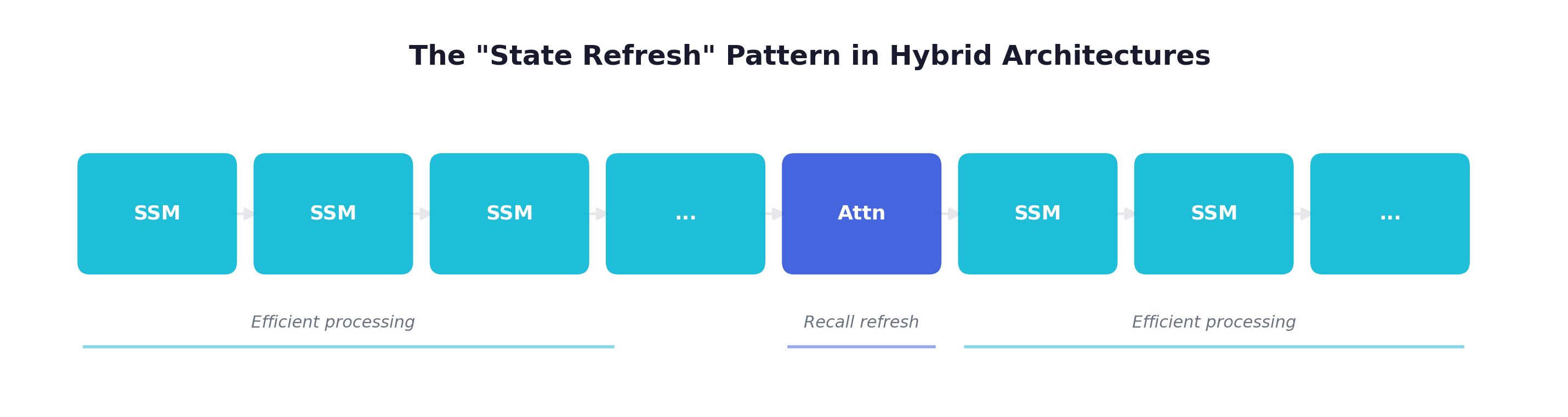
The SSM layers process the sequence efficiently, building up a compressed representation. But this compression is lossy — some information is inevitably lost or blurred. The attention layer acts as a “state refresh” — it allows the model to precisely retrieve information that may have been compressed or lost in the SSM state. The subsequent SSM layers then process this refreshed, more accurate information.
(4). Attention Type: Full vs. Sliding Window
- Full attention (Jamba): Maximum recall, but cost at each attention layer
- Sliding window (Samba): Cheaper ( cost), but only local recall
- Grouped-query (Falcon H1): Reduced KV cache while maintaining quality
The choice depends on whether you need global recall (exact retrieval from anywhere in the sequence) or just local recall (sharp pattern matching in recent context).
Comparison Table
| Model | Efficient Layer | Attention Type | Ratio | Scale | Notable |
|---|---|---|---|---|---|
| Jamba | Mamba | Full | 1:7 | 52B (12B active) | 256K context |
| Zamba2 | Mamba | Shared full | Weight-shared | 7B | Parameter efficient |
| Samba | Mamba | Sliding window | ~1:1 | 7B | Strong benchmarks |
| Falcon H1 | Mamba-2 (SSD) | GQA | Mixed | 7B | Reasoning focus |
| Griffin | Gated LRU | Sliding window | Mixed | 2-14B | Google’s approach |
| RecurrentGemma | Griffin | Local | Mixed | 2-9B | Production ready |
The Inference Advantage: Concrete Numbers
Even with some attention layers, hybrids offer significant inference advantages:
Pure Transformer (all 32 layers are attention):
- Per-token KV cache cost: — every layer stores K, V
- At 100K context: ~32 × 2 × 100K × d_head × n_heads ≈ 6.4 GB KV cache
Hybrid (25% attention = 8 attention layers, 75% SSM = 24 layers):
- KV cache: only for 8 layers → 8 × 2 × 100K × d_head × n_heads ≈ 1.6 GB
- SSM state for 24 layers: 24 × d_inner × d_state ≈ negligible (~1 MB)
- Total: ~1.6 GB — a 4x reduction in memory
The SSM state is negligible compared to the KV cache at any reasonable context length. The memory savings translate directly to larger batch sizes and lower latency.
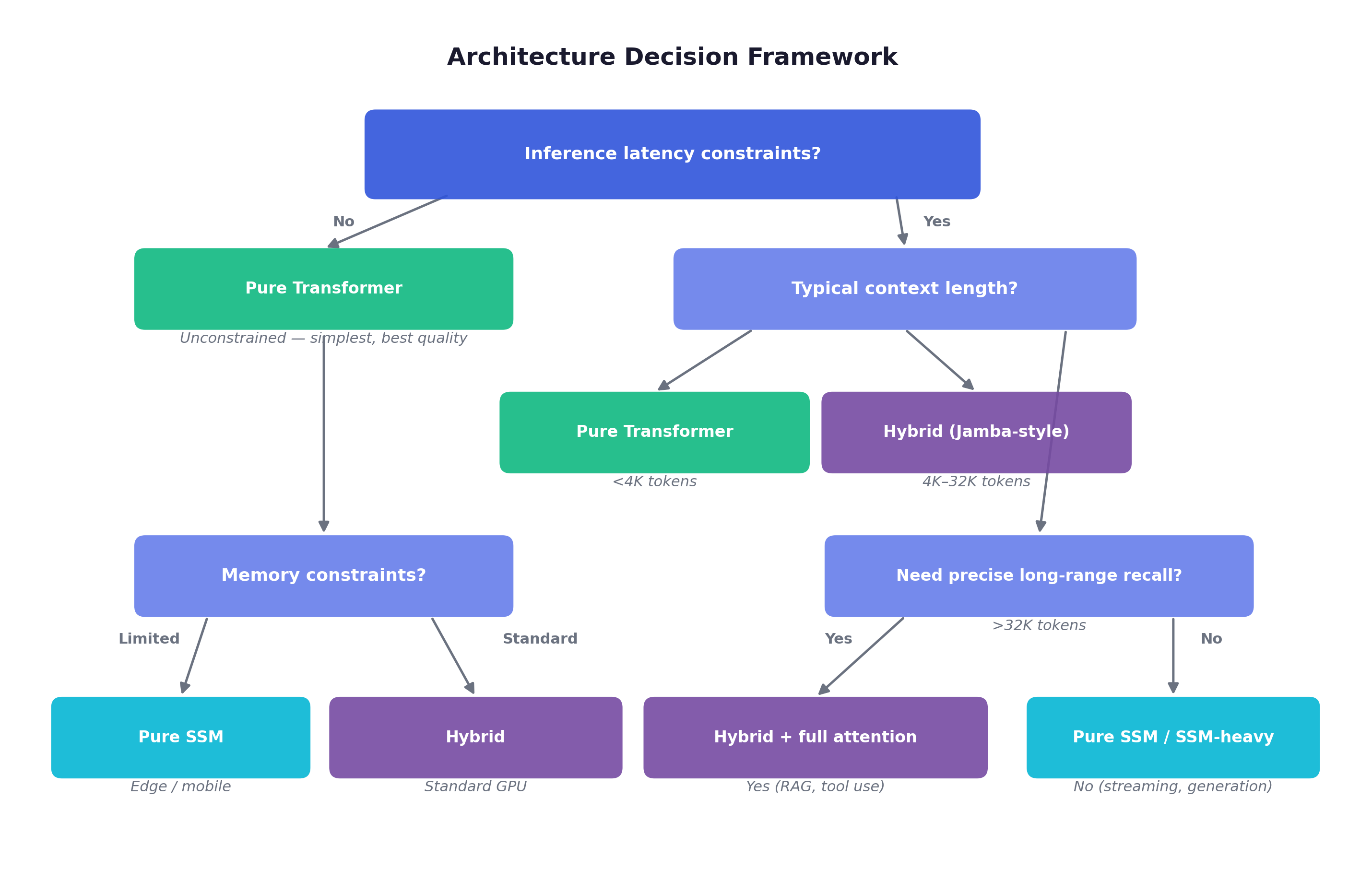
When to Use What
| Scenario | Recommended Architecture |
|---|---|
| Short context (<4K), quality-critical | Pure Transformer |
| Medium context (4K-32K), balanced | Hybrid (Jamba-style) |
| Long context (32K-256K) | Hybrid with sliding window (Samba-style) |
| Streaming / real-time | Pure SSM or SSM-heavy hybrid |
| Memory-constrained (edge, mobile) | Pure SSM (Falcon Mamba) |
| Maximum recall needed (RAG, tool use) | Transformer or attention-heavy hybrid |
| Agentic RL with long rollouts | Hybrid — SSM for speed, attention for tool-use recall |
8. Practical Implications and Choosing the Right Architecture
The Rollout Bottleneck, Revisited
One reason I got interested in this topic is its direct connection to the most demanding workload in modern AI: agentic reinforcement learning training.
In my RL infrastructure survey, I noted that 80-90% of RL training time is spent on sample generation (rollouts). The SSM efficiency gains become very concrete here:
| Token | Transformer (50K tokens) | SSM — Mamba/Mamba-2 (50K tokens) |
|---|---|---|
| Token 1 | Attend to 1 token → 1 unit | ≈ 1 unit |
| Token 1,000 | Attend to 1,000 tokens → 1,000 units | ≈ 1 unit |
| Token 50K | Attend to 50K tokens → 50,000 units | ≈ 1 unit |
| Total | 1.25 billion | 50K |
That’s a 25,000x reduction in total compute for the generation phase. Even after accounting for SSM layers being more expensive per-operation than individual attention steps, and the fact that real models have many layers and the comparison isn’t perfectly apples-to-apples, the potential speedup for long-context generation is striking.
Concrete Impact on Agentic RL Training
Consider a Slime-style agentic RL setup where:
- The agent interacts with a code execution environment
- Average rollout length: 30K tokens (prompt + multiple tool calls + reasoning)
- Training requires 100K rollouts per update
With a pure Transformer (7B scale):
- KV cache per rollout: ~4 GB
- Maximum batch size limited by GPU memory → fewer parallel rollouts
- Generation dominates training wall-clock time
With a hybrid (75% SSM, 25% attention):
- State per rollout: ~1 GB (4x less KV cache + small SSM state)
- 4x larger batch size → better GPU utilization
- Generation time scales near-linearly with rollout length instead of quadratically
This isn’t purely hypothetical — companies like Cartesia are already building SSM-based models specifically for real-time, long-context applications, and Falcon H1 uses a Mamba-2 hybrid backbone.
The Recall-Efficiency Frontier
The central tension in the field can be visualized as a Pareto frontier:
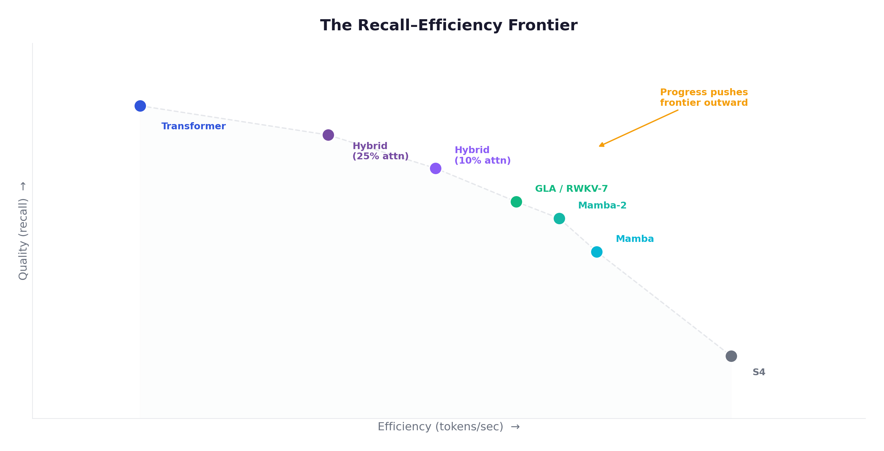
Each architecture occupies a point on this frontier. The field’s progress has been to push the frontier outward — getting more quality for the same efficiency, or more efficiency for the same quality.
Key developments pushing the frontier:
- Mamba (2023): Selective parameters dramatically improved quality for pure SSMs
- Mamba-2 (2024): Hardware-efficient SSD pushed throughput without quality loss
- Hybrid architectures (2024-2025): Mixing in minimal attention recovered recall capability
- GLA, RWKV-7 (2024-2025): Better gating/update rules closed the quality gap further
Decision Framework
Ecosystem Maturity
One practical consideration that often dominates architecture choices: software ecosystem maturity.
| Architecture | Frameworks | Pre-trained Models | Custom Kernel Support |
|---|---|---|---|
| Transformer | PyTorch, JAX, TensorRT, vLLM | Abundant (Llama, GPT, Qwen, etc.) | Flash Attention, PagedAttention |
| Mamba | mamba-ssm (CUDA), Triton | Mamba (130M-2.8B), Falcon Mamba 7B | Mamba CUDA kernels |
| Mamba-2 | mamba-ssm v2 | Limited | SSD Triton kernels |
| Hybrid | Framework-dependent | Jamba, Zamba, Falcon H1 | Mixed (attention + SSM kernels) |
The Transformer ecosystem is vastly more mature. Choosing an SSM or hybrid architecture means fewer pre-trained checkpoints, less optimized serving infrastructure, and more custom engineering. This gap is closing — particularly as frameworks like vLLM add Mamba support — but remains significant in 2025.
9. The Road Ahead
Open Questions
(1). Scaling Beyond 14B
No pure subquadratic model has been trained above ~7B parameters. Can the SSM advantages hold at 70B+? The theory seems to suggest yes — the efficiency gains become even more pronounced at scale, since the vs gap widens. But no one has demonstrated it empirically. The cost of training at this scale is prohibitive for most labs, and the companies that can afford it (OpenAI, Google, Anthropic, Meta) have invested heavily in Transformer infrastructure.
(2). Adaptive State Sizes
Current SSMs use fixed-size states (d_inner × d_state). Could we have adaptive state sizes that grow when the content demands it? Log-linear attention is one approach: the state grows logarithmically with sequence length, maintaining a Pareto-optimal position between fixed-state RNNs and full-state attention.
(3). The Role of Attention in Reasoning
There’s emerging evidence that attention may be particularly important for chain-of-thought reasoning, where the model needs to refer back to intermediate results. Consider a 10-step math derivation: the model must reference step 3’s result when computing step 7. SSMs’ exponentially decaying state may struggle here, while attention can precisely retrieve any previous step.
If this is true, the optimal hybrid ratio may be task-dependent:
- Math reasoning: more attention needed (precise reference to intermediate steps)
- Code generation: SSM-heavy for speed, attention at verification points
- Conversational: mostly SSM (recent context dominates)
- Long-document QA: hybrid with full attention for retrieval
(4). Hardware Co-Design
Mamba-2’s success came partly from aligning the computation with tensor cores. Future architectures may be designed in tandem with hardware:
- GPUs (H100/H200): Favor large matrix multiplications → chunked SSD fits well
- TPUs: Favor different operation patterns → may enable different SSM designs
- Emerging architectures (Groq, Cerebras): May favor different primitives entirely
- The “best” architecture may be hardware-dependent
(5). Convergence with Control Theory
SSMs have deep roots in control theory and signal processing. As the field matures, we may see more cross-pollination:
- Better initialization from control-theoretic analysis (beyond HiPPO)
- Stability guarantees from Lyapunov theory (provably stable recurrences)
- Optimal filtering connections (Kalman filter → SSM with learned noise model)
- Observer design principles for state estimation in noisy sequences
The Arc of Progress
| Year | Architecture | Key Properties |
|---|---|---|
| 2017 | Transformer | , parallelizable, powerful |
| 2021 | S4 | / , dual forms, but time-invariant |
| 2023 | Mamba | / , content-aware selection |
| 2024 | Mamba-2 | / , tensor cores, SSM=Attention duality |
| 2024 | Hybrids | amortized, best of both worlds |
| 2025 | Convergence | Architecture is secondary; data, recipe, and scale matter more |
| 2026 | UPDATE: Mamba-3 | TODO: Complex dynamics (data-dependent RoPE), MIMO, new Pareto frontier |
My sense is that within a few years, the attention-vs-SSM debate will feel as settled as the CNN-vs-RNN debate in NLP was by 2018. The likely answer: use the right tool for each layer.
The most interesting architectures going forward will probably be ones that make this choice adaptively — attending precisely when recall demands it, flowing efficiently when it doesn’t. Not as a static design choice made once at architecture time, but potentially as a dynamic decision at each layer, for each sequence, at each position.
The question, as I see it, isn’t whether Transformers will be replaced. It’s whether each layer in a model needs to be a Transformer. Increasingly, the answer seems to be no — and the layers that aren’t are getting faster every month.
References
Foundational Papers
- S4: Efficiently Modeling Long Sequences with Structured State Spaces (Gu et al., 2021)
- Mamba: Linear-Time Sequence Modeling with Selective State Spaces (Gu & Dao, 2023)
- Transformers are SSMs: Generalized Models and Efficient Algorithms Through Structured State Space Duality (Dao & Gu, 2024)
- Mamba-3: Improved Sequence Modeling using State Space Principles (Gu et al., 2026)
Architecture Variants
- Jamba: A Hybrid Transformer-Mamba Language Model (AI21 Labs, 2024)
- GLA: Gated Linear Attention Transformers with Hardware-Efficient Training (Yang et al., 2023)
- RWKV: Reinventing RNNs for the Transformer Era (Peng et al., 2023)
- RetNet: Retentive Network: A Successor to Transformer for Large Language Models (Sun et al., 2023)
- Falcon Mamba: The First Competitive Attention-free 7B Language Model (TII, 2024)
- HGRN2: Gated Linear RNNs with State Expansion (Qin et al., 2024)
Hybrid Architectures
- RecurrentGemma: Moving Past Transformers for Efficient Open Language Models (Google, 2024)
- Samba: Simple Hybrid State Space Models for Efficient Unlimited Context Language Modeling (Microsoft, 2024)
- Zamba: A Compact 7B SSM Hybrid Model (Zyphra, 2024)
Surveys
- The End of Transformers? On Challenging Attention and the Rise of Sub-Quadratic Architectures (2025)
- Efficient Attention Mechanisms for Large Language Models: A Survey (2025)
Implementations and Resources
- state-spaces/mamba — Official Mamba/Mamba-2
- state-spaces/s4 — S4 reference code
- The Annotated S4 — Excellent S4 walkthrough
- Mamba: The Hard Way — Detailed Mamba implementation guide
- tiiuae/falcon-mamba-7b — Falcon Mamba weights
- RWKV/RWKV-LM — RWKV implementation
- Cartesia AI Blog — SSM deployment insights